
Parameter estimation in arterial spin labeling MRI: Comparing the four phase model and the buxton model with fourier transform
Abstract
This paper presents a comparison between two algorithms that analyze and extract brain perfusion parameters from pulsed arterial spin labeling (ASL) MRI images. One algorithm is based on a Four Phase Single Capillary Stepwise (FPSCS) model, which divides the time course of the signal difference between the control and labeled images into four phases. The other algorithm utilizes the Buxton model and Fourier transformation (FTB). Both algorithms were implemented on MATLAB to extract the bolus arrival time (BAT) and the cerebral blood flow (CBF). In-vivo brain MRI images acquired at 4T from health volunteers were used in the comparison. Results indicated that the FTB algorithm had similar estimations of the BAT and CBF compared to the FPSCS model when the time signals are sufficiently sampled, but the former had faster processing speed while the FPSCS method provides additional information.
Keywords
Magnetic Resonance Imaging; Arterial Spin Labeling; bolus arrival time; cerebral blood flow
Introduction
Arterial Spin Labeling (ASL) is a non-invasive magnetic resonance imaging (MRI) method to quantify tissue perfusion. Perfusion gives a measure of the effectiveness of the blood circulation to provide oxygen and nutrients to the tissue and the ability to remove waste products. Unlike in positron emission tomography (PET) or contrast-enhanced MRI, ASL uses endogenous blood water tagged with radio frequency (RF) pulses as tracers. The method is attractive because no externally injected contrast agent is required. As a result, it can be performed repeatedly without additional side effects and costs. ASL has been used to study a variety of cerebrovascular diseases, neurodegenerative disorders, multiple sclerosis, as well as functional activation in healthy and pathological subjects. Measurement of perfusion is also useful for studying pathological conditions in heart, lung and bone marrow (1-14).
A major component in ASL MRI is to obtain quantitative perfusion values based on the measured MRI data. Perfusion is typically quantified by cerebral blood flow (CBF), which can be derived from the ratio of cerebral blood volume (CBV) and the mean transit time (MTT) (15-18). Another parameter, bolus arrival time (BAT), which characterizes the exact time when the labeled blood reaches the imaging slice, is also important because it is also an important parameter for study aging and certain neurological disorders (3,5,19).
Many algorithms have been published for extracting these parameters from ASL MRI time series data. This study will focus on two algorithms. The first algorithm is the Four Phase Single Capillary Stepwise (FPSCS) model (16). This model takes into account the transit effects and restricted permeability of capillaries to blood water. It divides the time duration of the tagged blood in the region of interest (ROI) and takes into account the arrival time of labeled blood water at the ROI, transit time through the arteries of the region, and the duration of the bolus of labeled spins. This sophisticated algorithm can yield estimate with less errors in the least-squares sense than the conventional model. The second algorithm estimates brain perfusion parameters by utilizing Fourier Transform (20). This algorithm uses a classical Buxton model (15) and applies a Fourier transform to extract the BAT and CBF. The algorithm was compared with a non-linear least square fitting algorithm, which shows that it provides similar accuracy on the BAT and CBF estimates.
The purpose of this research is to compare the FPSCS model and the FTB method on the same sets of ASL brain images. Specifically we will investigate how much the two algorithms deviate in their estimates of BAT and CBF. In addition, the computational efficiency of the two algorithms is also evaluated. Comparisons are expected to help identify appropriate algorithms for different application scenarios. This work is developed based on a preliminary report in a conference proceeding in (21).
Theory
Patients
In ASL, two sets of images are acquired: the tagged image, Mtag, is acquired after the arterial blood water in a labeling region (typically on the neck and below the brain image slices) is inverted by a radio-frequency pulse. The tagged water will travel up to the brain image slices. After a preset delay after tagging, the brain region will be imaged using an echo-planar or fast gradient echo sequence; the other image, Mctrl, is a control image acquired similarly as the tagged image but without the RF tagging or with a ″dummy″ tagging. The difference between the tagged image and the controlled image, in principle, comes from the perfusion of the labeled blood water. In practice, a time series of images are acquired, which correspond to different time delays, or inversion time. The time series provides the time-dependent dynamic information which is the basis for perfusion kinetic modeling and parameter estimation.
Next we briefly review the two ASL parameter estimation algorithms that will be examined in this paper.
Four Phase Single Capillary Stepwise (FPSCS) Mothod
In this model, the time duration of the ASL signal is divided into four phases with respect to the arrival time of labeled blood water at the region of interest (tA or BAT), transit time through the arteries of the region (tex), and the duration of the bolus of labeled spins (τ). The four phases are illustrated in Figure 1.

The FPSCS model also incorporates the capillar y permeability. Therefore, the signal difference of the tagged and controlled ASL time series can be presented as

where t is time, f is the CBF, and PS represents the capillary permeability.
Phase 1: Transit Phase

The tagged blood has not reached the arteries yet in this phase. Since the tagged blood is not present in the ROI, the signal difference is zero.
Phase 2: Arterial Phase (tA<t≤tA + tex)

where M0 denotes the equilibrium magnetization, α is the labeling efficiency, and R1b is the longitudinal relaxation rate of water in blood. During this phase, the tagged blood is still in the arteries. So the signal depends on the portion of the labeled blood in the voxel.
Phase 3: Arterial-Capillary Transitional Phase (Tex<t≤Tex+τ, where Tex= tA+tex)
During this phase, the labeled blood partially entered the capillary bed for exchange. The ASL signal in this phase comes from three parts: the blood in the arterial space, ΔMa(t), the contribution from intra-capillary space, ΔMc(t), and the contribution from the extra-capillary space, ΔMe(t). The total signal is therefore

Models for each of the components are given in the reference (16).
Phase 4: Capillary Phase (t>Tex+τ)
In this phase, all of the labeled blood water has entered the capillary bed for exchange. The contribution from arterial space vanishes. Therefore, only the last two components in Eq. [4] are left and

The parameters are determined by a nonlinear least-squares fitting between the model and the acquired experimental data, i.e., ΔM(tn).
The Buxton model and Fourier transformation (FTB)
According to the Buxton model, the signal difference between the control and tagged image is modeled as
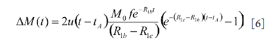
where u(t) is the Heaviside unit step function, R1b is the longitudinal relaxation rate of water in blood, and R1e is the longitudinal relaxation rate of perfused tissue. Generally, M0, R1e, and R1b either have to be measured, or are assumed to take typical values from literature. Therefore, the two parameters of interest, bolus arrival time (tA) and blood flow (f), are to be estimated from the measured signal differences. To do so, a Fourier transform is applied to Eq. [6] to yield
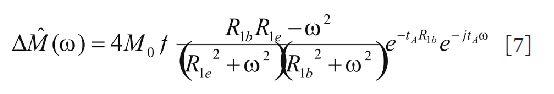
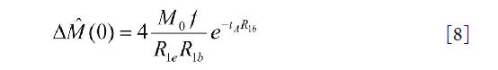
where ω is the time frequency variable. It is clear from Eq. [7] that the DC component
and the phase of the spectrum in Eq. [7]

Therefore the slope of the phase change with respect to the frequency is determined by tA. Collectively, Eq. [8] and [9] provide a mean to estimate BAT (tA) and blood flow(f) after M0, R1app, and R1b are known or assumed. Unlike the FPSCS model, this method is analytical because no iterative model fitting is required.
Methodology
To compare the two algorithms, both were implemented in MATLAB (Mathworks, Natick, MA, USA) to extract BAT and CBF parameters. In-vivo brain ASL data were acquired from healthy volunteers. Two types of perfusion analysis were conducted on the acquired images. The first was to analyze the brain image voxel by voxel in a ROI and generate a BAT map and a CBF map. Comparisons were then performed on the corresponding maps. The second was to analyze the average parameters in an ROI from a ″super″ voxel generated by spatially averaging the voxel signal intensities within the ROI.
Data Acquisition
Volunteers were scanned at a 4T MR unit (Bruker Medical Systems, Best, Erlangen) using an 8-channel head array coil. Interleaved tagged and control images were acquired using a fast 3D-GRASE sequence. Three-dimensional images were collected with a repetition time TR=3000 ms and an echo time TE=23.28 ms. For comparison, two sets of data were acquired: the first at 6 different inflow times (TI=400, 600, 1000, 1600, 2000, and 2600 ms) in the time series (dataset 1); the second at 13 different inflow times (TI=70, 200, 500, 800, 1000, 1200, 1400, 1600, 1800, 2000, 2200, 2400, and 2600 ms) in the time series (dataset 2). The k-space data matrix was 128Χ34, with a field of view of 300Χ150 mm (in plane resolution, 2.34Χ8.82 mm), and a slab thickness of 100 mm (slice thickness 4.7 mm). The number of signal average (NSA) in all acquisitions was 8. Twenty two axial slices were acquired to cover the entire hemispheric areas of brain. These raw control and labeled images were reconstructed at 128Χ128 points before the subtraction were taken to generate the ASL image. No registration of any kind was applied to the time series.
Data Analysis
Parameter Estimating using the FPSCS Model
The model fitting was based on a Simplex algorithm (22). This program requires the following parameters to be inputted to start the processing: image size, image frame acquisition time in the time series (tn), the time series of ASL images as defined in Eq. [1], and a mask to define the ROI. In the first step, the program calculated and extracted parameters such as signal intensity for each voxel at different time samples, estimated arrival time, and estimated bolus duration. In the second step, these initial parameters were used in the model fitting to extract other parameters. The output of the model fitting includes: BAT, CBF, permeability (PSv), and a theoretical signal intensity curve according to the model and fitting parameters.
Parameter Estimating using the FTB Method
As in the FPSCS method, the analysis using the FTB method was first performed on a voxel-by-voxel basis. To start, the acquired ASL time series, ΔMa(tn), was interpolated to N data points using a cubic spline model. The interpolation is necessary since the original time series normally contains less than 15 data points which makes Discrete Fourier Transform (DFT) less reliable. The interpolated time series were then inputted to an M-point DFT. After proper shift, the M spectrum points ΔM^ (m) were uniformly sampled in the frequency range of [–π, π). To use Eq. [9], it is useful to recognize that for the continuous-time frequency,
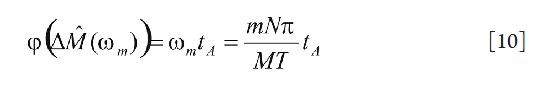
where T is the total duration of the time series. One potential problem in using Eq. [10] is the phase wrapping, since in computers all phase must be wrapped to [–π, π). For large BAT, the phase term is Eq. [10] could be potentially larger than π and therefore be wrapped to a negative phase. In this study, the problem was addressed by using a judicial choice of N and M for a given T. To improve the estimate, several lower frequency data points were used to estimate BAT and an average is taken. This is because lower-frequency spectrum points normally have higher signal-to-noise (SNR) ratio. For a ROI, the twenty voxels with the highest BATs were taken to determine the average BAT.
Another problem in using FTB method is the value of the equilibrium magnetization, M0. Without a given value for M0, the exact value for the CBF cannot be determined based on Eq. [8]. Measuring M0 in vivo is not straightforward due to flow contributions and relaxations. In the current study, it was assumed that M0 is uniform within an ROI, which is a reasonable assumption for brain tissues. The perfusion maps obtained under this assumption were therefore only relative. To facilitate comparison, a global scaling was applied to the map obtained from the FTB method so that the average difference in the two CBF maps is minimized. In addition, in both the FTB method and the FPSCS method, R1b and R1e took the same values measured by a conventional slice-selective inversion recovery acquisition.
Comparison between the FPSCS method and the FTB method
For both time series, the BAT and CBF maps for an ROI were generated and compared. The average values for the ROI were also list and compared. In addition, the theoretical dynamic ASL signals according to each model with the fitted parameters were drawn and compared. The total time taken to process the data by each method was recorded in MATLAB. The processing efficiencies of the two algorithms were compared based on the time spent.
Results
Figure 2 shows a representative brain image slice (difference image) from dataset 1, with an ROI highlighted on the left image. On the right graph, the average ROI signal intensity, i.e., that of the "super"-voxel, is shown in the solid red curve. The dashed blue curve represents the theoretical concentration curve generated by the FPSCS model according to the fitted model parameters. The two vertical lines mark the estimated BAT by the FTB method (solid red vertical line) and by the FPSCS method (dashed blue vertical line). As shown, there were noticeable differences in the estimated BATs in this case: 0.53 second and 0.36 second, respectively. This was possibly due to the insufficient time samples in the first dataset. However, the estimated CBFs by the two methods were very close: 248.8 and 247.6 (ml blood/min/100 ml tissue) by the FTB method and the FPSCS method, respectively.

The estimated BAT maps and the CBF perfusion maps by the two methods are shown in Figure 3. Note that in the FTB method, the background region was masked out to save processing time. Therefore the two BAT maps on top showed different background contrast. Similar to the result from the ROI analysis, the two BAT maps contained difference. However, it did not seem to significantly impact the perfusion parameter estimation. As indicated by the bottom row, these two CBF maps agreed well with each other.

A quantitative comparison in terms of the average BAT, average CBF, and the processing time for an ROI is listed in Table 1. As shown, the FTB method was faster than the FPSCS method in this example.
| Average BAT (s) | Average CBF (ml blood/min/100 ml tissue) | Processing Time (s)FPSCS | |
| FPSCS | 0.36 | 255.0 | 19 |
| FTB | 0.49 | 241.0 | 10 |
Next we present the analysis result of a representative slice from the ASL time series with 13 time samples (dataset 2). Figure 4 shows the brain image slice with the highlighted rectangular ROI, and the associated BAT analysis result, similar to the one shown in Figure 2. Note that in this example, the model curve and the measured time variation were matched to a higher degree, and the two BAT estimates were very close to each other.

A quantitative comparison of the two methods in terms of the average parameters for dataset 2 is shown in Table 2. The result showed that average perfusion estimates by the two methods were within 5% with each other. However, processing time of the FPSCS method in this test was significantly longer, partially due to the slower convergence in model fitting with more time samples.
| Average BAT (s) | Average CBF (ml blood/min/100 ml tissue) | Processing Time (s) | |
| FPSCS | 0.46 | 94.9 | 87 |
| FTB | 0.59 | 100.5 | 10 |
Disussion
The results showed that excellent accordance has been found between the 3D perfusion parametric maps from ASL-MRI with the use of FTB and FPSCS methods. In contrast to the FPSCS, implementation of FTB is much simpler. With shorter processing time, 3D flow and BAT maps of human brain can be obtained immediately after the data acquisition to enable a real time display. However, the FPSCS method could generate additional parameters in addition to the BAT and CBF shown in this study. These parameters provide valuable information about permeability of the capillaries.
A general observation in the study was that the FTB tended to overestimate the BAT while the FPSCS may underestimate the BAT. However, there did not seem to be systematic bias in the estimate of the relative CBF by either method. The estimated BAT and CBF maps often contained many noisy spikes. This is primarily due to the fact that the difference images are noisy, an inherent characteristic of the ASL signals with relatively low SNRs. In addition, closer check of the time course of individual voxels revealed that many did not show the inflow of the tagged blood water. Spatial filtering could improve the robustness against the noise, but may come at a cost of loss of fine features in the perfusion map. The current study was limited in that no ground truth was available to evaluate the accuracy of the methods. Moreover, statistical comparisons of various kinds may yield more insights about the methods.
Acknowledgements
This work was supported in part by the US National Science Foundation under Award number 0748180. Any opinions, findings and conclusions or recommendations expressed in this material are those of the author(s) and do not necessarily reflect those of the National Science Foundation.
References
- Herman P, Trbel H, Hyder F. Multi-modal measurements of CBF, CMRO2, and pO2 to determine oxygen back flux from blood to brain: Implications for fMRI. Proc Intl Soc Mag Reson Med 2003;11:125.
- Wang J, Alsop DC, Song HK, et al. Arterial transit time imaging with flow encoding arterial spin tagging (FEAST). Magn Reson Med 2003;50:599-607.[LinkOut]
- Asllani I, Habeck C, Scarmeas N, et al. Multivariate and univariate analysis of continuous arterial spin labeling perfusion MRI in Alzheimer's disease. J Cereb Blood Flow Metab 2008;28:725-36.[LinkOut]
- Detre JA, Alsop DC. Perfusion magnetic resonance imaging with continuous arterial spin labeling: methods and clinical applications in the central nervous system. Eur J Radiol 1999;30:115-24.[LinkOut]
- Du AT, Jahng GH, Hayasaka S, et al. Hypoperfusion in frontotemporal dementia and Alzheimer disease by arterial spin labeling MRI. Neurology 2006;67:1215-20.[LinkOut]
- Gonzalez-At JB, Alsop DC, Detre JA. Cerebral perfusion and arterial transit time changes during task activation determined with continuous arterial spin labeling. Magn Reson Med 2000;43:739-46.[LinkOut]
- Golay X, Hendrikse J, Lim TC. Perfusion imaging using arterial spin labeling. Top Magn Reson Imaging 2004;15:10-27.[LinkOut]
- Williams DS. Quantitative perfusion imaging using arterial spin labeling. Methods Mol Med 2006;124:151-73.[LinkOut]
- Wong EC, Buxton RB, Frank LR. Quantitative perfusion imaging using arterial spin labeling.Neuroimaging Clin N Am 999;9:333-42.[LinkOut]
- Lanting C. Perfusion imaging using arterial spin labeling: A study of continuous and pulsed arterial spin labeling. Groningen: University of Groningen;2005.
- Love T. Arterial spin labeling: University of Michigan;2007.
- Petersen ET, Zimine I, Ho YC, et al. Non-invasive measurement of perfusion: a critical review of arterial spin labelling techniques. Br J Radiol 2006;79:688-701.[LinkOut]
- Wang J, Zhang Y, Wolf RL, et al. Amplitude-modulated continuous arterial spin-labeling 3.0-T perfusion MR imaging with a single coil: feasibility study. Radiology 2005;235:218-28.[LinkOut]
- Ma T, Yuan J, Yeug KWD, et al. Kinetic study of bone marrow perfusion using arterial spin labeling. Proc Intl Soc Mag Reson Med 2010;19:3202.
- Buxton RB, Frank LR, Wong EC, et al. A general kinetic model for quantitative perfusion imaging with arterial spin labeling. Magn Reson Med 1998;40:383-96.[LinkOut]
- Li KL, Zhu X, Hylton N, et al. Four-phase single-capillary stepwise model for kinetics in arterial spin labeling MRI. Magn Reson Med 2005;53:511-8.[LinkOut]
- Parkes LM. Quantification of cerebral perfusion using arterial spin labeling: two-compartment models. J Magn Reson Imaging 2005;22:732-6.[LinkOut]
- Petersen ET, Lim T, Golay X. Model-free arterial spin labeling quantification approach for perfusion MRI. Magn Reson Med 2006;55:219-32.[LinkOut]
- Chao LL, Buckley ST, Kornak J, et al. ASL perfusion MRI predicts cognitive decline and conversion from MCI to dementia. Alzheimer Dis Assoc Disord 2010;24:19-27.[LinkOut]
- Guenther M. Analytical parameter estimation in arterial spin labeling time series by fourier transformation. Proc Intl Soc Mag Reson Med 2005;13:1136.
- Pham V, Zhu XP, Li KL, et al. Parameter estimation in arterial spin labeling MRI: comparing the Four Phase model and the Buxton model with Fourier transform. Conf Proc IEEE Eng Med Biol Soc 2009;2009:4791-4.[LinkOut]
- Press WH, Flannery BP, Teukolsky SA, et al. Numerical recipes. New York. Cambridge Univ Press; 1986.

