

Exploring a new method for quantitative sodium MRI in the human upper leg with a surface coil and symmetrically arranged reference phantoms
Introduction
The interest in sodium-23 (Na) magnetic resonance imaging (MRI) is quickly growing since the discovery that sodium can be stored in the skin and muscles without being osmotically active (1-3). Non-invasive quantification of the amount of sodium stored in muscle is now possible at 3T and has been validated against direct measurement of sodium in amputated human legs (4). Almost all Na MRI studies presenting a quantification of the tissue sodium concentration (TSC) in humans made use of external reference phantoms to transform the image intensity into a sodium concentration (see the supplementary discussion in the supplementary information online). Most of these studies performed a quantification of the TSC in the brain or in the leg muscles by use of birdcage (volume) coils. These coils have the advantage that they offer a relatively spatially homogeneous transmit field (B1+) and coil sensitivity pattern (B1−), so that all reference phantoms are excited in a relatively similar manner and lie in a similar coil sensitivity pattern. In contrast, non-volume coils such as transmit and receive (Tx/Rx) surface coils offer a spatially highly inhomogeneous transmit field as well as a coil sensitivity that decreases rapidly with the distance from the coil. On the other hand, the advantage of a surface coil is that it can target regions of the body such as the upper leg muscles, which are not accessible by volume coil.
In this study, we explore a new method for TSC quantification in the human upper leg muscles with a Tx/Rx surface coil that excites all reference phantoms in a similar manner and allows them to lie in a similar coil sensitivity pattern thanks to a symmetrical arrangement of the phantoms with respect to the coil. This method should in theory lead to a similar distribution of flip angles in the difference reference phantoms as well as a similar spatial pattern of the coil sensitivities through all the phantoms. Consequently, even if the B1+/B1– corrections are not exact, the relative signal intensities between phantoms should not be biased. The first aim of this study was to perform a validation test of our method and to assess its reproducibility in phantoms as well as in the upper leg muscles of humans. As far as we know, this is the first study that makes use of reference phantoms symmetrically arranged with respect to the coil and the first 23NA MRI study on the upper leg.
To perform this study, we had access to an ultrashort echo time (UTE) 3-dimensional projection reconstruction sequences (3DPR), as well as to the standard two dimensional (2D) spoiled gradient echo sequence (GRE). The advantage of the UTE sequences lies in its very short echo time minimizes the effect of T2* relaxation, which tends to affect the signal to noise ratio (SNR) in a favorable manner. Moreover, minimizing the T2* relaxation is even more important for sodium MRI than for conventional MRI since the fast decay time constant of the sodium signal (T2f) is as small as 0.5–5 ms and represent a signal fraction Ff of about 60% (5). On the other hand, our isotropic UTE sequence was naturally unable to produce anisotropic voxels with a large through plane thickness (in order to increase the SNR). In many organs, thick anisotropic voxels could have been undesirable since thick voxels could have produced unwanted partial volume effects between different kinds of tissues. However, since the targeted organ in this study is the upper leg muscles, it is reasonable to admit that very thick voxels do not produce partial volume effect between muscles and other tissue, because of the linear geometry of the leg. This fact opens the possibility to use the standard GRE sequence with a very large slice thickness in order to perform sodium imaging. In fact, the GRE sequence suffers from its relatively large echo time as compared to the UTE sequence. But on the other hand, the very large slice thickness that is achievable with GRE may compensate the loss of signal due to its large echo time, relatively to the UTE sequence. It was therefore not clear to the authors if a protocol making use of a UTE sequence with a very short echo time (but a small voxel size) performed better for the tissue sodium quantification in the human upper leg than a protocol making use the a GRE sequence and a large slice thickness (but a larger echo time). As a second aim of this study, a comparison between two such protocols was performed.
Methods
Participants
Eleven healthy volunteers aged between 20 and 40 years were scanned to test the reproducibility of the method in the human upper leg. An additional volunteer was scanned to measure the in vivo parameters of the bi-exponential signal decay of sodium i.e., the fast decay time constant T2f, the signal fraction of the fast decaying component Ff, and the long decay time constant T2l. Exclusion criteria for the participants were: age younger than 18 years, incapacity to provide informed consent or a contra-indication to MR imaging (pacemaker, implanted metallic device, claustrophobia). The study was approved by the local ethical committee (Ethical Committee of the Canton de Vaud, Switzerland) and written informed consent was obtained from the participants.
Sodium coil and symmetrically arranged reference phantoms
Figure 1 displays the experimental apparatus. The antenna used in this study is shown in Figure 1A. It contained an excite and receive (Tx/Rx) sodium-tuned surface coil made of a single circular loop of 14 cm (RAPID Biomedical, Rimpar, Germany). The same antenna contained also a hydrogen tuned butterfly coil allowing the acquisition of hydrogen images.

All phantoms used in this study were made of commercially available plastic boxes filled with a 2% agar gel and a known and homogenous NaCl concentration, either 10, 20, 30 or 40 mmol/L. We used two different phantom sizes. To calibrate the sodium signal intensity in each scan, 12×8×2.5 cm3 Reference phantoms were placed inside the field of view (Figure 1F, right). We named these phantoms R10, R20, R30 and R40 according to their NaCl concentrations. To validate the method and asses its reproducibility, four 21×13×8 cm3 Validation phantoms with similar NaCl concentration were used. We named them V10, V20, V30 and V40 according to their NaCl concentrations (Figure 1F, left).
To place the reference phantoms in a symmetrical manner with respect to the sodium coil, a Plexiglas support was built so that the coil could be maintained flat while the reference phantoms were located under the coil (Figure 1B). Of note, for the use of the 2D GRE-protocol, only two reference phantoms could be used (R20 and R40) in order to be placed symmetrically with respect to the loop coil (Figure 1D). For the use of the 3D UT-protocol, four reference phantoms could be used (R10, R20, R30 and R40) and were placed as shown in Figure 1E. The coil and phantoms were placed on the scanner table with the spine-coil removed (Figure 1C). This set up allowed the volunteer to lie in supine position with their leg flat on the antenna and the feet entering first into the scanner. All phantoms experiments were performed by placing the validation phantoms on the center of the coil. In every scan, the apparatus was stacked to the right of the table and the z-coordinate (along the table axis) of the center of the coil was placed at the z=0 coordinate with respect to the isocenter. Doing so, the coil was placed at the same location in every scan.
MR protocol
All images were acquired on a 3T-whole-body MR system (Magnetom Prisma, Siemens Medical Systems, Erlangen, Germany) and all scans began with a fast low angle shot (FLASH) localizer. We make use of the following notation in this subsection: field of view (FoV), flip angle (FA), pixel band width (BW), turbo factor (TF), repetition time (TR), echo time (TE) and acquisition time (AT).
The sodium GRE-protocol was set with the following parameters: orientation transversal, FoV 300×300 mm2, slice thickness 33 mm, in plane resolution 64×64, BW 350 Hz/pix, TR 100 ms, TE 1.73 ms (minimum), FA 90°, averages 124 and AT 13 min 15 s. The resulting voxel size was 4.7×4.7×33 mm3. An asymmetric echo was used. The transmitter reference amplitude (vRef) was adjusted so that the signal acquired in the V20 phantom and averaged in a rectangular region of interest (ROI) was maximal. This ROI was chosen to be 4 pixels (18.8 mm) deep in the phantom to take the thickness of skin and fat of the volunteer into account, and to exclude the complex excitation pattern very close to the surface coil.
The parameters for the UTE-protocol were set as similar as possible to those of the GRE-protocol. Only the TE was minimized in order to take advantage of the UTE sequence. The parameters were: FoV 300×300×300 mm3, resolution 64×64×64, TR 100 ms, TE 0.197 ms, FA 90, BW 350 Hz/pix, AT 13 min 12 sec. The resulting voxel size was 4.7×4.7×4.7 mm3. The stack of 7 transversal planes equaled thus the slice thickness of 33 mm of the GRE-protocol (we neglected the difference of 0.19 mm). The acquisition time was also equal to the GRE-protocol’s (we neglected the 3 second difference). The 3-dimentional trajectory was a spiral phyllotaxis pattern with each readout starting immediately from the center of k-space (6,7) and 39.2% of the Nyquist rate was achieved. A rectangular non-selective excitation pulse was used and the pulse duration was minimized to 225 micro-seconds. A delay of 50 micro second allowed the coil to change from the emit- to receive-mode. Finally, the analog-digital-converter (ADC) was turned on 30 micro-seconds before the gradient ramp-up in order to prevent side effects of the switch of the ADC. The first point of the read-out was excluded (because it underestimated the signal) and the signal was read from the second point (22.3 micro second after the first point). Additionally, it was known that our ADC suffered of a delay of 5.12 micro second to switch on. A minimum echo time of 0.197 ms resulted.
In contrast to phantoms, additional anatomical images were acquired in the volunteers with a turbo spin echo sequence (TSE) prior to the sodium scan. The protocol parameters were as follow: orientation transversal, FoV 300×300 mm2, in plane resolution 128×128, slice thickness 4.5 mm, distance factor 4%, BW 228 Hz/pix, TR 3,120 ms, TE 88 ms (echo spacing 9.8 ms), FA 150°, echo train per slice 15, TF 9, number of slices 9 and AT 50 s. The resulting voxel size was 2.34×2.34×4.5 mm3. Of note, the space between the centers of each two consecutive slices was 4.7 mm and the middle slice was through the isocenter. The slices of the TSE sequence matched thus the planes of the 3D UTE sodium sequence, and the 7 middle slices of the TSE sequence covered the 33 mm thick slice of the GRE sodium sequence. All images were acquired in the same position as the sodium images so that all the images were registered without further post-processing.
Image reconstruction for the UTE sequence
The image reconstruction for the radial trajectory of the UTE sequence was implemented on Matlab 8.6 R2015b (The MathWorks Inc., Natick, MA). The data acquired along the radial trajectory were first interpolated on a three dimensional Cartesian grid before applying the conventional inverse Fourrier transform. A convolution-based interpolation was used with a Kaiser-Bessel convolution kernel. The density compensation was performed as explained in (8) (p. 516). First, an image with value 1 on the entire radial trajectory was gridded on the Cartesian grid. This leaded to a weight-map on the Cartesian grid. Then, the gridded values of the sodium images were point-wise normalized by the previously computed weight-map.
SNR comparison between the GRE and UTE protocols
A one-night scan of 64 consecutive acquisitions on the V20 phantom was performed for each of the GRE and UTE sequences. The 7 closest planes to the isocenter of the UTE images, which cover the 33 mm thick slice of the GRE sequence, were averaged to obtain 64 2-dimensional (2D) images. For both acquisitions (GRE and UTE), the 64 2D images were averaged to obtain a 2D average signal map. Similarly, the standard deviation over the 64 acquisition was computed for each voxel and resulted in a 2D standard deviation map. The SNR map was then computed for each protocol by dividing point wise the average signal map by the standard deviation map, and dividing the result by the square root of 64. The SNR maps of the UTE and GRE protocols were then compared as described in the statistical analysis section.
Measure of T2f and T2l
Four repeated scans were performed on a healthy volunteer with the UTE sequence and with the echo times 0.197, 0.397, 0.797 and 6.00 ms respectively. No correction of the sodium images was needed since only the signal relative intensity was important to determine the decay time constants. For each of the four scans, the signal intensity was averaged in ROIs drawn on the TSE images as described in the next subsection. The resulting four values were then fitted as a function of the echo times by the use a least-square bi-exponential fitting procedure. A value for T2f, T2l and the fraction of the fast decaying signal component (Ff) was obtained. The same procedure was applied to the reference phantoms present under the coil during this scan to estimate the corresponding T2f and T2l constants.
A similar experiment was also performed on the validation phantoms. The only two differences with the in vivo scan were that seven scans were performed (instead of four) with the respective echo times 0.197, 0.397, 0.797, 1.597, 3.197, 6.397 and 12.797 ms, and that the signal intensity was average in a rectangular ROI.
Quantification of the sodium concentration
In phantoms, the sodium images were corrected for the B1+ and B1− inhomogeneities in two different ways. One method used a variant of the double-flip angle method and is described in the supplementary information available online. We called this correction method the “flip-angle correction” in this article. The other method was a normalization of the sodium image by the average signal map computed with the 64 acquisitions in the V20 phantom (see the SNR comparison subsection). This correction method was called the “normalization-correction”. After the sodium image was corrected for B1+ and B1– inhomogeneities, the signal was averaged in a rectangular ROI. This rectangular region excluded every voxel lying higher that the picture row (or line) 44, numbered from the top of the picture, because they were too far from the coil to contain a reliable signal intensity. This rectangular region also excluded every voxel lying under that the picture row number 48 (close to the coil). The reason for that exclusion is that the detected signal intensity in those voxels was unreliable because the B1+/B1– correction methods failed very close to coil. The signal intensity (after correction) was then averaged and converted into a sodium concentration by a piecewise linear interpolation between the signal values of the reference phantoms.
In volunteers, the TSC was assessed in a similar way as in the phantom, but with two additional steps. The first one was to correct the signal intensity in the leg and in the reference phantoms because of their different T2*-decays. This was done using the estimation of the T2*-decay parameters of both compartments (leg and reference phantoms) measured as described in the previous sub-section, and by dividing the signal intensities of each compartment by its respective correction factor β2 defined in the supplementary information (the T1 relaxation effect was neglected, see the discussion section). The second additional step was to segment the leg muscle to average the signal intensity in it. The segmentation was done manually by drawing regions of interest on each T2-weighted image acquired with the TSE sequence. The muscles were included inside the segmentation while fat and bones were excluded. Additional exclusion regions were drawn on the T2-weighted images around the vessels of large caliber (detected as dark spots) and fat infiltrations (bright voxels). As explained above for phantoms, voxels of the row higher than 44 and lower than 48 were also excluded of the segmentation. The sodium signal intensity of the sodium corrected images was then averaged inside the segmented region for the TSC quantification. The 9 closest plans to the isocenter were considered for the TSC quantification with the UTE sequence. The average signal intensity in the muscles was then turned into a sodium concentration as for the phantoms. All the post processing was done with Matlab 8.6 R2015b (The MathWorks Inc., Natick, MA).
Validation and reproducibility study
To perform a validation test on the method, the four validation phantoms with known NaCl concentrations were scanned with the apparatus including the reference phantoms as described above and their sodium concentration was quantified. To assess the reproducibility of this method, each validation phantom was scanned 5 times. Before every scan, the phantom was taken out of the scanner, re-entered, the shimming was repeated and the frequency was calibrated. All the phantom experiments were done with the GRE and the UTE sequence for comparison.
In order to test the reproducibility on human volunteers, each protocol was performed two times in each volunteer and at the same site (i.e., the upper leg muscles). As a byproduct of these data, an in-vivo comparison between the GRE measurement against the UTE measurement could be performed.
Statistical analysis
The reproducibility of the phantom measurements was quantified by the coefficient of variation (CV) that we defined as the standard deviation of the 5 measurements divided by their average value. The accuracy of the method was quantified by the bias that we defined as the difference between the average of the five measurements and the known sodium concentration, and then divided by the known sodium concentration. Four biases and four standard deviations were thus obtained, one for each validation phantom. To asses if the biases of the method, as measure in the four validation phantoms, were significantly different from 0, a two tailed t-test was used on the five measurements.
To decide if the GRE sequence had a different SNR than the UTE sequence, the pixel-by-pixel difference between the two corresponding SNR maps was listed and a two-tailed t-test was performed to assess if the mean value of this list was significantly different from 0.
The reproducibility of the TSC measurements on volunteers was assessed by the mean relative difference between the first and the second measurement, that is, the magnitude of the difference divided by the average of both measurements. The bias between the GRE and the UTE measurements in volunteers was also assessed by the mean relative difference and its significance was assessed by a paired t-test. The Pearson-correlation between the UTE and GRE measurements in volunteers and the corresponding p-value were calculated with the function “corrcoef” of Matlab (The MathWorks Inc., Natick, MA).
To asses if the sodium signal decays measured in-vivo and in the reference phantoms were significantly better fitted by a bi-exponential model than a mono-exponential one, an F-test was applied as described in (9).
Any of these tests was considered as positive if the resulting P value was smaller than 0.01.
Results
Phantom experiment
Figure 2A and B display the signal mean intensity (on the V20 phantom) as a function of vRef for the GRE sequence resp. UTE sequence. We estimated from these curves that the optimal vRef was close to 90 V for the GRE sequence and close to 62 V for the UTE sequence.

Figure 3A displays the average signal map (of the 64 acquisitions) acquired on the V20 phantom with the GRE protocol, Figure 3B displays corresponding standard deviation map and Figure 3C displays the corresponding SNR map. Figure 3D displays average signal map acquired on the V20 phantom with the UTE protocol, Figure 3E displays corresponding standard deviation map and Figure 3F displays the corresponding SNR map. The voxel values of the picture row (or line) number 48 (considering the top row as row number 1) of both SNR maps is plotted in Figure 4. The SNR of the GRE protocol is larger on this picture row. By considering the SNR values of all voxels inside the phantom, the GRE sequence lead to an average SNR of 4.0 while this average was 1.5 for the UTE sequence (i.e., 2.7 times lower). This difference was statistically significant.


The results of the validation and reproducibility study performed on the phantoms are displayed in Table 1. All biases were significantly different from 0 [noted with an asterisk (*)]. The correction with the flip-angle method was feasible in the validation phantoms with the GRE protocol. It was however unreliable when using the UTE protocol because the SNR was not high enough. Only the normalization correction was used with the UTE protocol.

Full table
Figure 5A displays one of the sodium images acquired on the V20 phantoms with the GRE protocol. Figure 5B displays the corresponding corrected image (with the flip angle correction) and Figure 5C displays the signal intensity of the V20 phantom together with the signal intensity of the reference phantoms. The sodium concentration measured in this image was 18.0 mmol.

Figure 6A, B and C display the analog images of Figure 5 for the V20 phantom and with the use of the normalization-correction. It can be observed that the correction fails close to the coil. The sodium concentration measured in this image was 20.3 mmol/L. Figure S1 shows the line-plots of all columns of Figure 6A and displays the range of lines that were accepted for sodium quantification (i.e., lines 44 to 48 from the top of the picture).


Figure 7A, B, and C are the UTE counter parts of Figure 6A, B and C. The 9 closest plans to the isocenter were average to obtain these 2D images. The sodium concentration measured in this image was 20.4 mmol/L. A view of a coronal plane of the 3D image is displayed in Figure 8A and shows the four references phantoms. The corresponding corrected image (with the normalization correction) is displayed in Figure 8B.


Figure S2 displays the T2*-signal decays measured in the four validation phantoms together with the corresponding bi-exponential fits. The median value over the four phantoms of the measured decay parameters were 5.26 ms, 43.2 ms and 63.8% for T2f, T2l and Ff. The signal decays of all four phantoms were significantly better fitted with a bi-exponential than with a mono-exponential fit.

In vivo experiment
The in vivo measured sodium signal decay acquired in one of the additional volunteer is displayed in Figure S3A and was significantly better fitted with a bi-exponential model than with a mono-exponential one. For the fast decaying component, we measured a signal fraction Ff =23.9% with a time decay constant T2f =0.325 ms. We measured a long time decay constant T2l =12.5 ms. The reference phantoms in this experiment didn’t exhibit a bi-exponential decay, possibly because a too low SNR. However, a mono exponential fit on the signal decay of each reference phantom lead the following homogeneous results for the decay time constant: 13.5, 13.7, 13.8 and 13.4 ms. Figure S3B displays the in vivo signal decay together with the signal decay of each reference phantom.

In volunteers, the image correction with the flip-angle correction was not reliable for both the GRE and UTE images because the SNR was not sufficiently high. Therefore, only the normalization correction was achieved for in vivo acquisitions.
Figure 9A displays the sodium image acquired with the GRE protocol in a volunteer. Figure 9B displays the corresponding corrected image (with the normalization-correction) and Figure 9C displays the average sodium signal intensity of the leg together with the signal intensities of the reference phantoms. The TSC measured with the GRE protocol in this volunteer was 10.7 mmol. Figure S4A displays a T2-weighted image (fourth slice) of the volunteer’s leg together with the ROI and the region of exclusion used for the sodium quantification. Figure S4B shows the sodium image acquired with the GRE protocol together with the same ROI and region of exclusion as Figure S4A.


Figure 10A displays the sodium image acquired with the UTE protocol (average of the 9 closest plans to the isocenter) in another volunteer. Figure 10B displays the corresponding corrected image (with the normalization correction) and Figure 10C displays the average sodium signal intensity of the leg together with the signal intensities of the reference phantoms. The TSC measured with the UTE protocol in this volunteer was 11.1 mmol. Figure S5A displays a T2-weighted image (slice number 7) of the volunteer’s leg together with the ROI and the region of exclusion used for the sodium quantification. Figure S5B shows the sodium image acquired with the UTE protocol (plane number 7) together with the same ROI and region of exclusion as Figure S5A.


The reproducibility study on the 11 volunteers lead a mean relative difference (between the first and the second measurement) of 3.0% for the GRE protocol and of 3.7% for the UTE protocol. Both GRE measurements from each volunteer were average in order to obtain 11 TSC for the GRE-protocol. Similary, 11 TSC values were obtained for the UTE protocol and compared pairwise to those of the GRE protocol. The mean relative difference between both was 10% and was significant, but the Pearson correlation of these two paired sets of values was significant and equal to 79%.
Discussion
The main findings of our study are: (I) TSC quantification in the human leg muscles using sodium MRI and a surface coil with symmetrically arranged reference phantoms is reproducible in humans and in phantoms (II) the GRE-protocol leads to 2D images with a 2.7 times larger SNR than the UTE-protocol when compared for the same covered volume, (III) the quantification of the sodium concentration in phantoms is accurate when the UTE protocol is used on validation phantoms, but the quantification fails for small concentrations (10 mmol/L) when the GRE protocol is used.
The main potential limitation of our method is that the in-vivo measured sodium concentration may underestimates the true in-vivo sodium concentration because our values are roughly half of previously published values [see for example (10)]. The reason for this potential underestimation remains unclear as our method is accurate on phantoms (bias less than 10% for the UTE protocol with TE =0.197 ms). This underestimation (as compared to other studies) is maybe due to the inherent limitations of single loop surface coils because the TSC values measured in the leg muscles in other studies were all obtained with volume coils on the calves. Another possibility is that TSC may be lower in the upper leg than in the calves. This is to be explored by further 23NA studies since we is the first one performed on the upper leg, as far as we know. Another limitation of our study is the large bias (30%) affecting the GRE-protocol for the TSC estimations of small values (10 mmol/L for instance). A possible explanation may be that the low number of reference phantoms used in the GRE protocol do not allow to perform an accurate signal calibration. In fact, there are no 10 mmol/L reference phantoms in the GRE protocol, while there is one in the UTE protocol. This difference may explain that the UTE protocol does not suffer of the same bias as the GRE protocol.
As said in the method section, the T1 relaxation effect was neglected for the TSC quantification. We justify this by the fact that the T1-relaxation effect should, in the worst case, affect the image grey values (after normalization correction) by not more than 9%, which is small compared to the image noise. For this estimation, we considered the TR of 100 ms and some T1 estimates from the literature (11,12) for agar phantoms and muscle. Concerning the effect of the voxel size on the signal intensity, this should be canceled by our normalization correction if we assume that the voxel size affects the signal intensity by a multiplicative factor, which depends on the voxel volume.
The fast decay time constant of the sodium signal (T2f) is as small as 0.5–5 ms and represent a signal fraction Ff of about 60%, while the long decay time constant (T2l) is about 15–30 ms and contributes to about 40% of the signal (5). For that reason, sequences with trajectories starting immediately from the center of k-space, i.e., UTE sequences, are commonly preferred for sodium because they minimize the effect of the fast transverse relaxation. Sequences exhibiting ultrashort echo times and simultaneously covering the k-space efficiently and homogenously have been developed (13-19). They exhibited an improved SNR and an improved spatial resolution as compared to the standard GRE or even the traditional 3DPR sequences (19). On the other hand, in the recent years, some authors have been very successful in quantifying the TSC in the human leg muscles and skin by the exclusive use of the standard GRE sequence (4,10,20-22). This success may be partially explained by the fact that GRE takes advantage of the linear geometry of leg muscles. In fact, relatively thick transversal slices can be excited without causing partial volume effects between muscles and other tissues, and the signal can this way be increased proportionally to the voxel volume. The same is true for the skin of the leg, which has a planar geometry if the leg is lying on a plane surface. Moreover, by choosing the readout direction of the Cartesian trajectory to be parallel to the skin layer, the blurring along that direction caused by transverse relaxation during the echo is not a problem anymore for the quantification of sodium in the skin (22). In addition, quantification of TSC in a homogenous muscle mass with large region of interests (ROIs) does not need the high spatial resolution furnished by the mentioned sophisticated sequences. The GRE sequence may also have the following advantage over UTE sequences for that specific application. The 3D UTE sequences are usually isotropic, in which case thick planes with smaller in plane voxel size are not achievable in contrast to the 2D GRE. For the same in plane resolution as a 2D GRE, a 3D isotropic UTE sequence needs many planes, say N, to cover the unique thick slice of the GRE. Averaging the N planes from the UTE acquisition, we obtain an SNR that is proportional to the covered volume divided by  , while the GRE furnishes an SNR proportional to the covered volume itself. This represents an advantage of GRE over UTE for the sodium quantification in the upper leg, even if the same statement is not valid anymore in other organs with a non-linear geometry (i.e., where thick slices are not permitted because of partial volume). For these different reasons, it was not clear to the authors which protocol was better for TSC quantification in the leg muscles: the standard GRE sequence with a thick slice, or a 3DPR UTE sequence with an ultra-short echo time (UTE). This is the reason why a comparison between both protocols was performed. Ideally, any sequence used for TSC quantification in the leg should use both advantages: thick anisotropic voxels together with a UTE. Such sequences have been developed for sodium imaging (14,23) but are unfortunately not easily accessible since they are not commercially available.
The optimal amplitudes (vRef) of the excitation pulses of both sequences were found to be different and this can be explained as follow: the excitation pulse of the 2D GRE sequence was 2D selective, while the excitation pulse of the UTE sequence was spatially non-selective. Since the envelopes of both pulses were different but achieved the same flip angle, and since the flip angle is proportional to the area under the pulse envelope, the pulse amplitudes had also to be different as well.
Supplementary
Correction of the B1 + and B1 – inhomogeneities with the “flip-angle correction”
As a matter of fact, the signal intensity of a voxel is well approximated by the following expression when a gradient echo sequence is used:
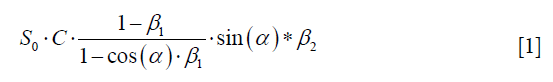
where α is the excitation angle in the voxel in question, 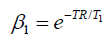 , β2 is the attenuation factor due to the T2* decay, S0 is proportional to the spin density, and C is a spatially dependent coil sensitivity factor. Of note, T1 depends on the voxel in question. For a mono-exponential decay, β2 has the form
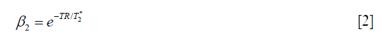
while for a bi-exponential decay with fast decay time constant T2f, long decay time constant T2l and a fraction of the fast decay component equal to Ff, the attenuation factor is

This attenuation factor depends also on the voxel through its three parameters. If we now acquire one image with a given excitation pulse amplitude leading to an excitation angle α, and then a second image with an excitation pulse amplitude higher of a factor q, the excitation angle of the second image will be q · α. If, for the same voxel, the signal intensities corresponding to the two images are noted S1 and S2, it follows from eq. [1] that their ratio leads
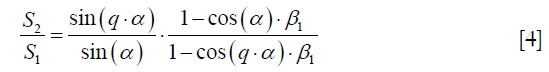
This function of α can be numerically inverted to find α, provided that the T1 of the voxel is known. If in addition the attenuation factor β2 is known, the factor S0 · C can be extracted from eq. [1]. From the reciprocal theorem and from the hypothesis that the transmit field is quasi static, we can assume that the coil sensitivity factor C is proportional to the B1+ field and thus proportional to α. Dividing S0 · C by α leads then in principle to a number that is only weighted by the spin density of the voxel. For q=2, this method is known as the “double flip angle method”.
We used the factor q=1.38 to corrected images acquired with the GRE sequence and the factor q=1.41 to corrected images acquired with the UTE sequence. To apply this correction to our images, we estimated the T1 of the agar phantoms with a previously published heuristic equation (11) and a temperature of 20°. We used a T1 of 28 ms. We approximated the T2* decay of the reference agar phantoms as bi-exponential decay with the parameters measured in our multiple echo experiment on the validation phantoms. We used also a bi-exponential model with the parameters measured in our multiple echo experiment on the volunteer to compute the β2 attenuation factor of muscles. And finally, we estimated the T1 of muscles from the previously published literature and we chose a value of 18.5 ms (12).
Supplementary discussion
As briefly stated in the introduction, transmit and receive (Tx/Rx) surface coils deliver a spatially inhomogeneous transmit field and coil sensitivity pattern. Consequently, reference phantoms are not excited in the same way and their signal intensities are weighted by different coil sensitivities, if they are not symmetrically arranged with respect to the coil. Some methods allow compensating for the B1+ inhomogeneities (24-27) as well as the B1− inhomogeneities (22,28). It is also possible to use adiabatic excitation pulses to obtain a spatially homogenous excitation independently of the B1+ inhomogeneities (29). But if these correction resp. excitation methods suffer of inexactitude, and if the reference phantoms are not symmetrically arranged with respect to the coil, the reference signal intensities from the phantoms, which serve for the calibration of TSC, are biased. We demonstrate on validation phantoms that the use of symmetrically arranged reference phantoms allows to overcome these limitations and represents an improvement in the measurement of TSC with Tx/Rx surface coils.
Concerning the choice of the optimal protocol for Na23 MRI of legs, it is important to note that the measure of T2f can only be measured with the UTE sequence. Since this value is used in the quantification of TSC in the leg muscles, even by the use the GRE sequence, the use of the UTE sequence in the method remains important even if its SNR is smaller than GRE’s.
In the intension of implementing NA MRI with a transmit and receive (Tx/Rx) surface coil at 3 Tesla (3T), the authors of the present article made a search on PubMed in order to get informed about the quantitative methods used until today. The following string was used for the search in the PubMed database: (sodium OR Na OR 23Na OR NA OR 23NA) AND (quantitative OR quantification OR content OR concentration) AND (MRI OR (MR imaging) OR (MR images) OR (magnetic resonance imaging)).
The authors did their best to detect all the articles presenting a method for quantitative sodium imaging in humans. It turned out that, up to very few exceptions, every reported method made use of external calibration phantoms with known sodium concentrations put inside the field of view during the scans, in order to transform the sodium signal intensity (SI) into a TSC. Methods that didn’t do so were of four kinds. In the first, the method made use of a single homogenous phantom of know sodium concentration that was scanned subsequently and served to normalize the sodium images as well as to transform the SI in TSC (30). The second method, used in the same study as the first method, was an improvement with a correction of the transmit field inhomogeneity by the use of a transmit field mapping technique (30). In the third, the SI of tissues in the acquired sodium image was calibrated on the SI of tissues of known sodium concentration acquired in previous scans [for example (31)]. And in the fourth method, the SI of cerebrospinal fluid (CSF) that was present in the field of view, with a known sodium concentration from previous studies, played the role of a reference phantom (32). Nevertheless, these four methods suffer of the following drawbacks. The first and third methods neglected the differences of coil loading present in different scans, while the fourth method suffers from the fact that sodium concentration of CSF varies with anatomical location (33). Concerning the second method, it is very time-consuming and could therefore not been applied to patient in the mentioned study. In a more often encountered method, the reference phantoms were scanned subsequently to the scan of the subjects (34-36). But even in this method, some other saline references were present in the field of view of the two scans (subject and references) in order to correct for the different coil loadings. In summary, up to the four mentioned exceptions that suffer of drawbacks due to the absence of reference phantoms during all scans, all methods for quantitative sodium MRI in humans make use of reference saline phantoms present in the field of view during the scan of the subjects. Reference phantoms for TSC quantification with sodium MRI are therefore important and, when a surface coil is used, the symmetrical arrangement of the phantoms with respect to the coil allows them to be excited in a similar manner and to lie in a similar coil sensitivity pattern.
Acknowledgments
We wish to thank Jessica Bastiaansen for her help in building agar phantoms. We also wish to thank the Swiss Society of Hypertension (Schweizerische Hypertonie Gesellschaft) for its financial help to this project.
Funding: This study was supported by the Swiss National Science Foundation (FN 320030-169191 and FN 32003B-149309).
Footnote
Conflicts of Interest: The authors have no conflicts of interest to declare.
Ethical Statement: The study was approved by the local ethical committee (Ethical Committee of the Canton de Vaud, Switzerland) and written informed consent was obtained from all volunteers.
References
- Titze J, Dahlmann A, Lerchl K, Kopp C, Rakova N, Schroder A, Luft FC. Spooky sodium balance. Kidney Int 2014;85:759-67. [Crossref] [PubMed]
- Wahlgren. Über die Bedeutung der Gewebe als Chlordepots. Arch Experim Pathol Pharmakol 1909;61:97-112. [Crossref]
- Rakova N, Juttner K, Dahlmann A, Schroder A, Linz P, Kopp C, Rauh M, Goller U, Beck L, Agureev A, Vassilieva G, Lenkova L, Johannes B, Wabel P, Moissl U, Vienken J, Gerzer R, Eckardt KU, Muller DN, Kirsch K, Morukov B, Luft FC, Titze J. Long-term space flight simulation reveals infradian rhythmicity in human Na(+) balance. Cell Metab 2013;17:125-31. [Crossref] [PubMed]
- Kopp C, Linz P, Wachsmuth L, Dahlmann A, Horbach T, Schofl C, Renz W, Santoro D, Niendorf T, Muller DN, Neininger M, Cavallaro A, Eckardt KU, Schmieder RE, Luft FC, Uder M, Titze J. (23)Na magnetic resonance imaging of tissue sodium. Hypertension 2012;59:167-72. [Crossref] [PubMed]
- Madelin G, Lee JS, Regatte RR, Jerschow A. Sodium MRI: methods and applications. Prog Nucl Magn Reson Spectrosc 2014;79:14-47. [Crossref] [PubMed]
- Delacoste J, Chaptinel J, Beigelman-Aubry C, Piccini D, Sauty A, Stuber M. A double echo ultra short echo time (UTE) acquisition for respiratory motion-suppressed high resolution imaging of the lung. Magn Reson Med 2018;79:2297-305. [Crossref] [PubMed]
- Piccini D, Littmann A, Nielles-Vallespin S, Zenge MO. Spiral phyllotaxis: the natural way to construct a 3D radial trajectory in MRI. Magn Reson Med 2011;66:1049-56. [Crossref] [PubMed]
- Bernstein MA, King KF, Zhou XJ. Handbook of MRI Pulse Sequences. Elsevier Science; 2004.
- Yuan J, Wong OL, Lo GG, Chan HH, Wong TT, Cheung PS. Statistical assessment of bi-exponential diffusion weighted imaging signal characteristics induced by intravoxel incoherent motion in malignant breast tumors. Quant Imaging Med Surg 2016;6:418-29. [Crossref] [PubMed]
- Kopp C, Linz P, Dahlmann A, Hammon M, Jantsch J, Muller DN, Schmieder RE, Cavallaro A, Eckardt KU, Uder M, Luft FC, Titze J. 23Na magnetic resonance imaging-determined tissue sodium in healthy subjects and hypertensive patients. Hypertension 2013;61:635-40. [Crossref] [PubMed]
- Nagel AM, Amarteifio E, Lehmann-Horn F, Jurkat-Rott K, Semmler W, Schad LR, Weber MA. 3 Tesla sodium inversion recovery magnetic resonance imaging allows for improved visualization of intracellular sodium content changes in muscular channelopathies. Invest Radiol 2011;46:759-66. [Crossref] [PubMed]
- Madelin G, Regatte RR. Biomedical applications of sodium MRI in vivo. J Magn Reson Imaging 2013;38:511-29. [Crossref] [PubMed]
- Boada FE, Gillen JS, Shen GX, Chang SY, Thulborn KR. Fast three dimensional sodium imaging. Magn Reson Med 1997;37:706-15. [Crossref] [PubMed]
- Nagel AM, Laun FB, Weber MA, Matthies C, Semmler W, Schad LR. Sodium MRI using a density-adapted 3D radial acquisition technique. Magn Reson Med 2009;62:1565-73. [Crossref] [PubMed]
- Irarrazabal P, Nishimura DG. Fast three dimensional magnetic resonance imaging. Magn Reson Med 1995;33:656-62. [Crossref] [PubMed]
- Gurney PT, Hargreaves BA, Nishimura DG. Design and analysis of a practical 3D cones trajectory. Magn Reson Med 2006;55:575-82. [Crossref] [PubMed]
- Pipe JG, Zwart NR, Aboussouan EA, Robison RK, Devaraj A, Johnson KO. A new design and rationale for 3D orthogonally oversampled k-space trajectories. Magn Reson Med 2011;66:1303-11. [Crossref] [PubMed]
- Lu A, Atkinson IC, Claiborne TC, Damen FC, Thulborn KR. Quantitative sodium imaging with a flexible twisted projection pulse sequence. Magn Reson Med 2010;63:1583-93. [Crossref] [PubMed]
- Konstandin S, Nagel AM. Measurement techniques for magnetic resonance imaging of fast relaxing nuclei. MAGMA 2014;27:5-19. [Crossref] [PubMed]
- Hammon M, Grossmann S, Linz P, Kopp C, Dahlmann A, Janka R, Cavallaro A, Uder M, Titze J. 3 Tesla (23)Na magnetic resonance imaging during aerobic and anaerobic exercise. Acad Radiol 2015;22:1181-90. [Crossref] [PubMed]
- Dahlmann A, Dorfelt K, Eicher F, Linz P, Kopp C, Mossinger I, Horn S, Buschges-Seraphin B, Wabel P, Hammon M, Cavallaro A, Eckardt KU, Kotanko P, Levin NW, Johannes B, Uder M, Luft FC, Muller DN, Titze JM. Magnetic resonance-determined sodium removal from tissue stores in hemodialysis patients. Kidney Int 2015;87:434-41. [Crossref] [PubMed]
- Linz P, Santoro D, Renz W, Rieger J, Ruehle A, Ruff J, Deimling M, Rakova N, Muller DN, Luft FC, Titze J, Niendorf T. Skin sodium measured with (2)(3)Na MRI at 7.0 T. NMR Biomed 2015;28:54-62. [PubMed]
- Konstandin S, Nagel AM, Heiler PM, Schad LR. Two-dimensional radial acquisition technique with density adaption in sodium MRI. Magn Reson Med 2011;65:1090-6. [Crossref] [PubMed]
- Insko EK, Bolinger L. Mapping of the radiofrequency field. J Magn Reson 1993;103:82-5. [Crossref]
- Akoka S, Franconi F, Seguin F, Le Pape A. Radiofrequency map of an NMR coil by imaging. Magn Reson Imaging 1993;11:437-41. [Crossref] [PubMed]
- Allen SP, Morrell GR, Peterson B, Park D, Gold GE, Kaggie JD, Bangerter NK. Phase-sensitive sodium B1 mapping. Magn Reson Med 2011;65:1125-30. [Crossref] [PubMed]
- Carinci F, Santoro D, von Samson-Himmelstjerna F, Lindel TD, Dieringer MA, Niendorf T. Characterization of phase-based methods used for transmission field uniformity mapping: a magnetic resonance study at 3.0 T and 7.0 T. PLoS One 2013;8:e57982. [Crossref] [PubMed]
- Haneder S, Konstandin S, Morelli JN, Nagel AM, Zoellner FG, Schad LR, Schoenberg SO, Michaely HJ. Quantitative and qualitative (23)Na MR imaging of the human kidneys at 3 T: before and after a water load. Radiology 2011;260:857-65. [Crossref] [PubMed]
- Ouwerkerk R, Weiss RG, Bottomley PA. Measuring human cardiac tissue sodium concentrations using surface coils, adiabatic excitation, and twisted projection imaging with minimal T2 losses. J Magn Reson Imaging 2005;21:546-55. [Crossref] [PubMed]
- Zaric O, Pinker K, Zbyn S, Strasser B, Robinson S, Minarikova L, Gruber S, Farr A, Singer C, Helbich TH, Trattnig S, Bogner W. Quantitative Sodium MR Imaging at 7 T: Initial Results and Comparison with Diffusion-weighted Imaging in Patients with Breast Tumors. Radiology 2016;280:39-48. [Crossref] [PubMed]
- Schepkin VD, Ross BD, Chenevert TL, Rehemtulla A, Sharma S, Kumar M, Stojanovska J. Sodium magnetic resonance imaging of chemotherapeutic response in a rat glioma. Magn Reson Med 2005;53:85-92. [Crossref] [PubMed]
- Wang C, McArdle E, Fenty M, Witschey W, Elliott M, Sochor M, Reddy R, Borthakur A. Validation of sodium magnetic resonance imaging of intervertebral disc. Spine (Phila Pa 1976) 2010;35:505-10. [Crossref] [PubMed]
- Haneder S, Konstandin S, Morelli JN, Schad LR, Schoenberg SO, Michaely HJ. Assessment of the renal corticomedullary (23)Na gradient using isotropic data sets. Acad Radiol 2013;20:407-13. [Crossref] [PubMed]
- Kalayciyan R, Wetterling F, Neudecker S, Haneder S, Gretz N, Schad LR. Bilateral kidney sodium-MRI: Enabling accurate quantification of renal sodium concentration through a two-element phased array system. J Magn Reson Imaging 2013;38:564-72. [Crossref] [PubMed]
- Ouwerkerk R, Bottomley PA, Solaiyappan M, Spooner AE, Tomaselli GF, Wu KC, Weiss RG. Tissue sodium concentration in myocardial infarction in humans: a quantitative 23Na MR imaging study. Radiology 2008;248:88-96. [Crossref] [PubMed]
- Ouwerkerk R, Jacobs MA, Macura KJ, Wolff AC, Stearns V, Mezban SD, Khouri NF, Bluemke DA, Bottomley PA. Elevated tissue sodium concentration in malignant breast lesions detected with non-invasive 23Na MRI. Breast Cancer Res Treat 2007;106:151-60. [Crossref] [PubMed]

