

Thermoacoustic elastography: recovery of bulk elastic modulus of heterogeneous media using tomographically measured thermoacoustic measurements
Introduction
Elastic modulus of tissue (1,2) is an important parameter in disease diagnosis, which can characterize tissue as soft or hard. Elastography for measuring tissue elastic modulus (2-9) is widely used as a supplementary diagnostic method for early detection and diagnosis of various diseases. At present, elastography has been implemented based on the contrast mechanism of ultrasound (US) imaging (3,10,11), optical coherence tomography (OCT) (4,12), magnetic resonance imaging (5,13) (MRI), or photoacoustic imaging (PAI) (6-9,14,15). These elasticity imaging techniques have been applied for the detection of liver fibrosis (16), breast cancer (17), and prostate cancer (18).
Here, we add a new method to the family of elastography based on the contrast mechanism of thermoacoustic tomography (TAT). TAT (19-25) is an emerging imaging technique based on the thermoacoustic (TA) effect, and provides high microwave contrast, high spatial resolution, and large penetration depth. Thermoacoustic elastography (TAE) has a wide range of potential medical applications, e.g., in the detection of cirrhosis, atherosclerosis, and cancers (25-27). In TAE, we reconstruct the bulk elastic modulus distribution by solving the TA wave equation based on the finite element method (FEM) without internal or external static stress or shear wave. We calculate acoustic pressure through the initial microwave energy loss and bulk elastic modulus distributions. The microwave energy loss and elastic modulus distributions are then iteratively updated until the error between the calculated and measured acoustic pressures meets a pre-set tolerance, or the number of iterations reaches a pre-set upper limit. Compared with optical coherence elastography and photoacoustic elastography, TAE has superior imaging depth. Compared to magnetic resonance elastography, TAE has higher resolution. Our TAE approach is tested and validated using both simulated and phantom experiments.
Methods
Image reconstruction algorithm
Key to the realization of TAE is an image reconstruction algorithm based on the FEM that simultaneously reconstructs tissue microwave energy loss and elastic modulus from tomographically measured TA signals.
Using the Newton’s law of motion, equation of continuity, and thermal elastic equation, the following time-domain TA wave equation can be derived (28):
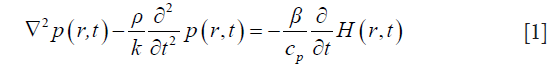
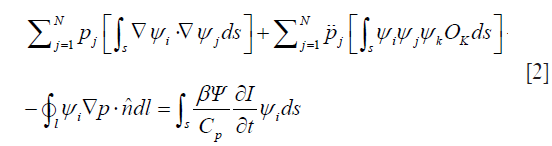
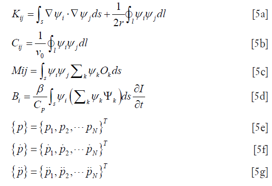
where p is the pressure wave, ρ is the mass density, t is the time, r is the spatial variable, K is the bulk elastic modulus, Cp is the specific heat capacity at constant pressure, and β is the thermal coefficient of volume expansion. H is the microwave excitation source term, which can be written as H=Ψ(r)I(t), where I(t) is the temporal illumination function and Ψ(r) is the absorbed energy density. To obtain Eq. [1], a homogeneous elastic reference medium is assumed with density, ρ=ρ0, and the bulk elastic modulus is denoted as K=ρv2, where v is the acoustic velocity. If we let  , and expand p and O as the sum of coefficients multiplied by a set of the basis function ψj and ψk—i.e., p=∑ψjpj and O=∑ψkOk— then the finite-element discretization of Eq. [1] is expressed as (29)
where  > is the unit normal vector.
The Bayliss-Turkel radiation boundary conditions are employed here (28):
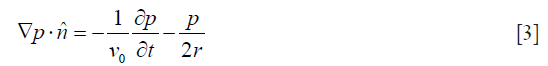
In both the forward and the inverse calculations, the unknown coefficients Ψ need to be expanded in a similar fashion to p, as a sum of unknown parameters multiplied by a known spatially varying basis function. Thus, Eq. [2] can be expressed in the following matrix form in consideration of Eq. [3],

where  are the values of the pressure and its derivatives at time t and the elements of the matrix are written
Here, the Newmark’s time stepping scheme is used for the discretization of the time dimension (28). To form an image from a presumably uniform initial guess of the microwave and mechanical property distributions, the iterative Newton’s method is used to update Ψ and O from their starting values. In this method, we Taylor expand p about an assumed (Ψ,O) distribution, which is a perturbation away from some other distribution, such that a discrete set of p values can be expressed as
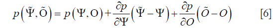
If the assume the microwave/mechanical property distributions are close to the true profiles, the left-hand side of Eq. [6] can be considered as the true data (observed or measured), and the relationship can be truncated to yield

where
and  and
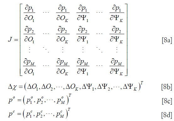
and  are the measured and calculated acoustic field data based on the assumed (p,Ψ) distribution data for i=1,2,…,M boundary locations. Ok and Ψk (k=1,2,…,K) are the reconstruction parameters for the elastic and microwave property profiles, respectively. In order to realize an invertible system of equations for Δχ, Eq. [7] is left multiplied by the transpose of J to produce

where regularization schemes are invoked to stabilize the decomposition of JTJ . I is the identity matrix, and λ is the regularization scheme combined Marquardt and Tikhonov regularization schemes. We have found that when λ=(po–pc)×trace[JTJ], the reconstruction algorithm generates best results, where trace[·] represents the trace of the matrix. The process now involves determining the calculated hybrid regularization-based Newton’s method to update an initial microwave/elastic property distribution iteratively via the solution of Eqs. [4,9] so that an object function composed of a weighted sum of the squared difference between computed and measured acoustic pressures can be minimized. The objective function F is given by

Considering the fact that US transducers and signal amplifiers have band-pass characteristics, we used the Butterworth band-pass filter module in the iterative process to improve the accuracy of reconstruction. The flowchart of the algorithm is shown in Figure 1. Before starting the calculation, we set microwave energy loss to 0.0001 a.u. and the elasticity coefficient to 1.90 GPa.

We conducted several simulations and phantom experiments to demonstrate the feasibility of the proposed TAE.
Numerical simulations
In the first simulation experiment, different contrast levels of elastic modulus between the targets and the background and microwave energy loss were used. A circular background region with the radius of 20 mm contained three circular targets (2 mm in radius each), positioned at 9, 2 and 6 o’clock, respectively. The bulk elastic modulus and microwave energy loss of the targets are listed in Table 1.

Full table
Similarly to the first simulation, a circular background region with a radius of 20 mm contained three circular targets positioned at 9, 2, and 6 o’clock with a radius of 5, 2, and 2 mm, respectively. The bulk elastic modulus, relative dielectric constant and conductivity of the targets are listed in Table 2. The microwave energy loss distribution was obtained by solving the electromagnetic wave equation. The microwave energy loss distribution obtained was then input into the algorithm for elastic modulus recovery. In the simulation setting, a plane wave at 3 GHz was incident along the x axis.

Full table
The reconstructed method was implemented based on a dual mesh scheme (30) with 1,584 nodes and 2,986 elements of coarse mesh and 6,153 nodes and 11,944 elements of fine mesh. Thirty iterations were required for a complete image reconstruction. Each iteration cost ~6 min on a 3.6 Ghz core processor with 20 GB memory.
Phantom experiments
The TAT system (19-21) we used to demonstrate the reconstruction method is schematically shown in Figure 2, where a coordinate system (X, Y, Z) is also depicted for reference. In this single transducer scanning experimental system, a pulsed microwave was generated from a custom-designed microwave generator (frequency: 3.0 GHz, bandwidth: 50 MHz, peak power: 70 KW, pulse duration: 750 ns). The microwave pulse was coupled into a rectangular waveguide and irradiated to a sample with less than 3.2 W/m2 power density at the sample surface by a horn antenna (114×144 mm2). A single-element unfocused transducer (V323, Olympus, central frequency: 2.25 MHz, nominal bandwidth: 1.35 MHz) was used to acquire the TA signal in a polyvinyl chloride tank filled with transformer oil for optimal microwave induced US signal transmission. TA signals at 180 positions were received via a step motor rotating the transducer around the sample over 360° in the X-Y plane. The signals were recorded by a data acquisition card (PCI4732, Vidts Dynamic) after amplified by a 58 dB amplifier (homemade, bandwidth: 250 kHz–2MHz).

In the phantom experiments, agar-based tissue-mimicking phantoms were used as the investigation samples. The elastic modulus was varied by changing the concentration of agar, while the microwave energy absorption was changed by adding 4% salt to the phantom. In the experiments, we made 2% (2.2 GPa elastic modulus), 4% (2.34 GPa elastic modulus) and 6% (2.43 GPa elastic modulus) agarose phantoms (3 mm in diameter each) with the transform oil background (1.90 GPa elastic modulus) for TAE. To improve the signal to noise (SNR), an average of 100 times was adopted during signal acquisition. The same finite element meshes as the simulations were used for the reconstruction using the experimental data.
In the first phantom experiment, a single target having 2% or 6% agarose was placed in the background. In the second phantom experiment, two cases were examined. In case 1, there were two 4% agarose targets. In case 2, there was a 2% agarose target and a 6% agarose target.
Results
Numerical simulations
In the first numerical simulation experiment, the anti-noise ability of the algorithm was also tested. For cases 1, 2, and 3, “measured” data without noise and with 20 and 10 dB SNR were used as the reconstructed input, respectively. In each case, the measured data was generated using the forward computation with the exact elastic modulus and microwave energy loss distribution at 180 receiving/detection positions equally distributed along the boundary of the circular background region.
Figures 3 and 4 show the reconstructed images for simulation cases 1–3. We see that both the microwave energy loss and elasticity can be well recovered for three targets having different contrast level relative to the background. When noise was added, we note that the microwave energy loss can still be reconstructed with high accuracy, while the impact of noise on the quality of elasticity image is notable. To further quantify these observations, Figure 4 is given to present the elastic modulus and microwave energy loss profiles along the two transects crossing the centers of target 1 and target 2. We can see that recovered values of the targets match well with the exact values. Mean reconstruction error is defined as the difference between the average reconstructed value and the exact value. For microwave energy loss and elastic modulus, they were found to be 0.15%/0.46%, 3.21%/5.49%, and 9.36%/12.1% for cases 1, 2, and 3, respectively.


In the second numerical simulation, the microwave energy loss distribution was not uniform because of the difference in dielectric properties of the targets and background. For the energy loss distribution (shown in Figure 4A), the middle of the target at 9 o’clock collapses, and the upper part of the target at 2 and the left part of the target at 6 o’clock are missing. For this complex distribution of microwave energy loss, the anti-noise ability of the algorithm was also tested. For cases 4, 5, and 6, “measured” data without noise and with 30 and 20 dB signal-to-noise ratio (SNR) were used as the input.
Figures 5 and 6 show the reconstructed images for simulation cases 4–6. Similarly, both microwave energy loss and elastic modulus distribution are well reconstructed. We can see that recovered values of the targets match well with the exact values. Although the energy loss distribution could not be accurately reconstructed in terms of the target shape due to the difference in dielectric constants, the recovered elastic modulus had no distortion. The mean reconstruction errors for microwave energy loss and elastic modulus were found to be 0.12%/0.11%, 2.17%/2.62%, and 5.43% /8.12% for cases 4, 5, and 6, respectively.


Phantom experiments
Figure 7 presents the reconstructed TAE images and image profiles using the phantom experiments of the first phantom experiment. In Figure 7, the elastic modulus of the first and second rows are 2.28 GPa, and the others are 2.48 GPa. From these images and image profiles, we see that our TAE algorithm has the ability to reconstruct energy density loss and elastic modulus simultaneously. The recovered shape and size of target agree well with the actual ones, and the mean error of the reconstructed elastic modulus was estimated to be less than 9.96% compared to the exact value.

The recovered TAE images (Figure 8) from the second phantom experiment are shown in Figure 8A,B,E,F, while the reconstructed elastic modulus, microwave energy loss and elastic modulus profiles are given in Figure 8C,D,G,H. We note that the error of recovered elastic modulus for the two 2.34 GPa targets is less than 9.7% for case 1, while for case 2 the reconstruction error for the 2.43 and 2.28 GPa targets are less than 11.22% and 12.74%, respectively.

Discussion
The goal of this study is to explore a simple methodology of elastic modulus reconstruction based on conventional TAT. On the basis of the results of simulation and phantom experiments presented above, it is clear that the image reconstruction algorithm described in this paper is feasible. It has been demonstrated that the reconstructed images can provide both qualitative and quantitative information about the targets in terms of their location, sizes, shape, microwave, and mechanical property values. These observations and the quantitative nature of the reconstructed images are further confirmed by the elastic modulus profiles provided.
From Figures 3-6, we can see that both elastic modulus and microwave energy loss distribution of the three targets with different contrast are accurately reconstructed. We note that the accuracy for the elastic modulus reconstruction is lower than that for the microwave energy loss especially when the SNR is reduced.
The reconstructed elastic modulus given in Figures 7 and 8 shows a good agreement with the exact value. It is worth noting that the computational time for TAE image reconstruction is long at present. We plan to speed up the reconstruction process using GPU-based parallel computing.
Conclusions
In summary, we have demonstrated a TAE approach that allows the simultaneous recovery of elastic modulus and microwave energy loss density using both simulated and experimental data. We plan to apply this TAE approach to in vivo studies, e.g., for cirrhosis detection in the near future.
Acknowledgements
Funding: This research was partially supported by the University of Electronic Science and Technology of China, and the National Natural Science Foundation of China (61701076 and 11674047).
Footnote
Conflicts of Interest: The authors have no conflicts of interest to declare.
References
- Majumdar S, Lin J, Link T, Millard J, Augat P, Ouyang X, Newitt D, Gould R, Kothari M, Genant H. Fractal analysis of radiographs: assessment of trabecular bone structure and prediction of elastic modulus and strength. Med Phys 1999;26:1330-40. [Crossref] [PubMed]
- Ophir J, Cespedes I, Ponnekanti H, Yazdi Y, Li X. Elastography: a quantitiative method for imaging the elasticity of biological tissues. Ultrason Imaging 1991;13:111-34. [Crossref] [PubMed]
- Ophira J, Cespedes I, Garra B, Ponnekanti H, Huang Y, Maklad N. Elastography: ultrasonic imaging of tissue strain and elastic modulus in vivo. European Journal of Ultrasound 1996;3:49-70. [Crossref]
- Schmitt J. OCT elastography: imaging microscopic deformation and strain of tissue. Opt Express 1998;3:199-211. [Crossref] [PubMed]
- Muthupillai R, Ehman RL. Magnetic resonance elastography. Nat Med 1996;2:601-3. [Crossref] [PubMed]
- Glatz T, Scherzer O, Widlak T. Texture Generation for Photoacoustic Elastography. Journal of Mathematical Imaging and Vision 2015;52:369-84. [Crossref]
- Hai P, Yao J, Li G, Li C, Wang LV. Photoacoustic elastography. Opt Lett 2016;41:725-8. [Crossref] [PubMed]
- Liu Y, Yuan Z. Multi-spectral photoacoustic elasticity tomography. Biomed Opt Express 2016;7:3323-34. [Crossref] [PubMed]
- Wang Q, Shi Y, Yang F, Yang S. Quantitative photoacoustic elasticity and viscosity imaging for cirrhosis detection. Applied Physics Letters 2018;112:211902. [Crossref]
- Zaleska-Dorobisz U, Kaczorowski K, Pawluś A, Puchalska A, Inglot M. Ultrasound Elastography – Review of Techniques and its Clinical Applications. Adv Clin Exp Med 2014;23:645-55. [Crossref] [PubMed]
- Sigrist RMS, Liau J, Kaffas AE, Chammas MC, Willmann JK. Ultrasound Elastography: Review of Techniques and Clinical Applications. Theranostics 2017;7:1303-29. [Crossref] [PubMed]
- Kennedy BF, Kennedy KM, Sampson DD. A Review of Optical Coherence Elastography: Fundamentals, Techniques and Prospects. IEEE J Sel Top Quantum Electron 2014;20:272-88. [Crossref]
- Mariappan YK, Glaser KJ, Ehman RL. Magnetic resonance elastography: A review. Clin Anat 2010;23:497-511. [Crossref] [PubMed]
- Zhao Y, Chen C, Yang S, Xing D. Mechanical evaluation of lipid accumulation in atherosclerotic tissues by photoacoustic viscoelasticity imaging. Opt Lett 2016;41:4522-5. [Crossref] [PubMed]
- Guo H, Chen Q, Qi W, Chen X, Xi L. In vivo study of rat cortical hemodynamics using a stereotaxic-apparatus-compatible photoacoustic microscope. J Biophotonics 2018.e201800067. [Crossref] [PubMed]
- Sandrin L, Fourquet B, Hasquenoph JM, Yon S, Fournier C, Mal F, Christidis C, Ziol M, Poulet B, Kazemi F, Beaugrand M, Palau R. Transient elastography: a new noninvasive method for assessment of hepatic fibrosis. Ultrasound Med Biol 2003;29:1705-13. [Crossref] [PubMed]
- Itoh A, Ueno E, Tohno E, Kamma H, Takahashi H, Shiina T, Yamakawa M, Matsumura T. Breast Disease: Clinical Application of US Elastography for Diagnosis. Radiology 2006;239:341-50. [Crossref] [PubMed]
- Cochlin DL, Ganatra RH, Griffiths DFR. Elastography in the Detection of Prostatic Cancer. Clin Radiol 2002;57:1014-20. [Crossref] [PubMed]
- Chi Z, Zhao Y, Yang J, Li T, Zhang G, Jiang H. Thermoacoustic tomography of in vivo human finger joints. IEEE Trans Biomed Eng 2018. Epub ahead of print. [Crossref] [PubMed]
- Zhao Y, Chi Z, Huang L, Zheng Z, Yang J, Jiang H. Thermoacoustic tomography of in vivo rat brain. Journal of Innovative Optical Health Sciences 2017;10:1740001. [Crossref]
- Chi Z, Zhao Y, Huang L, Zheng Z, Jiang H. Thermoacoustic imaging of rabbit knee joints. Med Phys 2016;43:6226. [Crossref] [PubMed]
- Xu F, Ji Z, Chen Q, Yang S, Xing D. Nonlinear Thermoacoustic Imaging Based on Temperature-dependent Thermoelastic Response. IEEE Trans Med Imaging 2019;38:205-12. [Crossref] [PubMed]
- Cui Y, Yuan C, Ji Z. A review of microwave-induced thermoacoustic imaging: Excitation source, data acquisition system and biomedical applications. J Innov Opt Health Sci 2017;10:1730007. [Crossref]
- Okawa S, Hirasawa T, Kushibiki T, Ishihara M. Image reconstruction of the absorption coefficients with l 1-norm minimization from photoacoustic measurements. Quant Imaging Med Surg 2015;5:78-85. [PubMed]
- Zheng Z, Huang L, Jiang H. Label-free thermoacoustic imaging of human blood vessels in vivo. Applied Physics Letters 2018;113:253702. [Crossref]
- Picot PA, Thornton MM, Steinberg DA. Thermoacoustic system for analyzing tissue. Google Patents; 2012.
- Wang B, Zhao Z, Liu S, Nie Z, Liu Q. Mitigating acoustic heterogeneous effects in microwave-induced breast thermoacoustic tomography using multi-physical K-means clustering. Applied Physics Letters 2017;111:223701. [Crossref]
- Yao L, Guo G, Jiang H. Quantitative microwave-induced thermoacoustic tomography. Med Phys 2010;37:3752-9. [Crossref] [PubMed]
- Jiang H. Photoacoustic tomography. CRC Press, 2014.
- Gu X, Xu Y, Jiang H. Mesh-based enhancement schemes in diffuse optical tomography. Med Phys 2003;30:861-9. [Crossref] [PubMed]

