
Robust principal component analysis in optical micro-angiography
Introduction
Microvascular imaging and quantification have attracted great interest in the field of medical imaging. Through the observations of changes in micro-vasculature and blood flow, diagnoses and therapeutic monitoring of many medical conditions that have vascular involvements can be benefitted. A few examples are: onset of atheroma, which is characterized by degeneration of arterial wall and arteriosclerosis at later stage (1); microcirculatory dysfunction, which is considered as a key pathogenesis of severe sepsis and septic shock (2); study of microvascular invasion and hypoxia of tumor (3), etc.
Realizing the importance of microvascular imaging, many research groups have been in pursuit for new and improved micro-angiography imaging techniques. Each technique, however, suffers from a significant tradeoff between resolution and field of view in living tissue imaging. Optical coherence tomography (OCT) is a three-dimensional (3D) imaging technique that can provide non-invasive, high-resolution cross-sectional images in real time (4,5). As a high-resolution functional extension to OCT, OCT-angiography (OCTA) (6-8) offers rapid, safe, non-invasive and cost-effective solution to imaging depth-resolved microcirculation down to capillary level, which has recently found its way to clinical translation, for example in ophthalmology (9-11).
Optical micro-angiography (OMAG) is introduced based on the observations of complex signal fluctuations, which are hypothesized to be related to moving erythrocytes within functional blood vessels (12-17). Due to the fact that scattering elements behave differently in static and moving (blood flow) regions, appropriate digital filtering of the OCT signals can distinguish blood flow signal from static tissue background, achieving blood flow mapping for microcirculatory tissue beds. There are many different algorithms to contrast blood flow signals from the OCT measurements, such as speckle intensity variance, phase variance, and complex signal analysis (8). This paper focuses on the OMAG complex signal analysis, which is also the main imaging modality throughout the discussion of this paper.
The analysis starts with the complex signal, following the Fast Fourier Transform (FFT) of spectral signal from Fourier-domain OCT. In OCTA/OMAG imaging protocol, it is required to scan the same tissue location repeatedly over time (i.e., repeated A-scans, or M scan) in order to build a time series of A-scan OCT signals, from which the signal fluctuation is extracted to represent the blood flow signal. Thus, the resulting complex OCT signal is a 2D matrix of a depth M-scan. Since the OCT probe beam is highly (randomly) scattered inside the blood vessels, blood flow signal can be extracted from the complex M-scan signal via an appropriate filter.
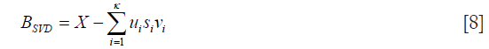
The most recent development in OMAG complex signal analysis relies on Eigen decomposition (ED) (18,19), which requires the formation of covariance matrix (XXT) from 2D space-time complex matrix signal, X. Since the formation of covariance matrix, XXT, can cause loss of precision [Läuchli matrix as an example (20)], singular value decomposition (SVD) is employed as an alternative technique in dynamic signal filtering (21). Furthermore, traditional PCA (including SVD and ED) techniques are sensitive to outliers, i.e., the principal components can easily be skewed by a few corrupted frames, due to severe sample motion that causes decorrelation between frames, and by tail-noise effect where speckle intensity varies greatly between frames.
With the recent development in linear algebra and computing, principal component analysis (PCA) [ED (22) and SVD] has been adopted on ultrasound angiography; robust principal component has been adopted in magnetic resonance, and X-ray computed tomography (21). This paper introduces readers to PCA methods for OMAG, and presents an improved algorithm, called robust PCA (RPCA). This RPCA technique is capable of extracting blood flow signal in capillaries with higher blood flow signal-noise ratio, and significantly reduces blood vessels’ tail-noise and motion-induced artifacts.
Background theory for PCA in OMAG
The PCA, by definition, is a statistical procedure that converts a set of observations on (possibly correlated) variables into a set of linearly uncorrelated new variables. Each new variable (described by the Eigen vector), called principal component, is a linear combination of the original (and possibly correlated) variables. This idea is important in OMAG, or OCTA in general, since most pixels containing static signal are highly correlated over a small-time window, while however is not the case for blood flow signal and noise.
In OMAG, PCA separates static and slow-moving signal data (highly correlated across the time frames), from uncorrelated signal such as blood flow, speckles and noise signal via linear-regression filter (18,19). This can be done by assuming that most of the signal comes from static scatters, and secondly, by assuming that the pixels containing static signal are highly linearly correlated (or at least has higher degree of correlation in comparison to the variations in blood flow and noise) within the observing time-window.
For example, we start the analysis by considering an OMAG M-scan complex data signal, X(z,t):

where s is the static signal, b is the blood signal, and n is the electronics/background noise. This complex data is usually expressed in matrix form, Xz,t, which has nz rows of spatial pixels (A-scan) × nt columns of time frames:
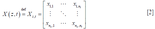
where nz is the index for discrete depth axis, and nt is the index of discrete time axis. For simplicity, we further assume that static signal is invariant over the observing time-window, but blood flow and noise. This assumption ensures that, over time, pixels containing static signals would have low variance across repeated frames, whilst pixels containing blood flow signals will appear sparse.
In PCA, the repeated A-scans form a data matrix that consists of nz (axial pixels) observations with nt (repeated frames) variables. Our objective is to find a set of linear combinations of temporal frames (variables), and decompose this set into the principal components. In simple case, the first PCA component (labelled as ‘1st PC’ in Figure 1) reconstructs exactly the static signal, since the frame are strongly correlated across spatial/depth pixels (observations). Blood flow and noise signal can then be reconstructed from the other components, i.e., second to nt-th principal components, as they are mostly uncorrelated between frames. An example of blood flow analysis using PCA is shown in Figure 1, where nz-pixel intensity between two repeated frames are plotted in log-scale for visual presentation. From our assumption about signal correlation across repeated frames, pixel containing static signal can be seen as data points adjacent to the first principal component (the 1st PC); and pixel containing blood flow signal can be seen as data points with high variance on second principal component (the 2nd PC). This analysis can also be generalized to higher dimensions, i.e., nt repeated frames.

In most cases, the general assumption holds that pixels (observations) containing static signals are dominant and are highly correlated across the slow-time (repeated nt frame). However, in real case scenario, static signals are not perfectly stationary across repeated frames due to random scattering event (speckle artifact) and tissue motion (motion artifact). These artifacts are generally considered to be outliers (see Figure 1), which can skew the principal components and produce unwanted results. For example, the first PC would attempt to reduce the variance from the outliers, thus making static signals appear to be dynamic. RPCA is therefore introduced in order to solve this problem regarding outliers.
Taking together, there are undoubtedly many techniques to achieve the separation between static and blood flow signals in complex signal analysis, but we will only discuss the development of RPCA for OCTA and compare RPCA with traditional PCA (which includes ED and SVD) in this paper. Although different techniques exist for different purposes in the field of OMAG, they all aim to recover a highly correlated signal (static or slow-moving signal) from uncorrelated signal (i.e., dynamic blood flow). PCA and RPCA analysis are discussed in each section below. A summary of each technique is shown in Table 1.

Full table
ED and linear regression filter
The first technique in our PCA discussion is the ED, using multi-ensemble data matrix. In general, the data matrix is pre-processed before the analysis, i.e., constructing covariance/correlation matrix from a 2D space-time data, X. The choice between covariance and correlation matrix is entirely subjective, and depends on different techniques and purposes. For most of our applications in OMAG, employing either covariance or correlation matrix would yield similar results (i.e., the linear regression or 1st PC passes through the origin in most cases). The covariance matrix,

where E is the expectation value, superscript *T is the conjugate (Hermitian) transpose,
In practice, we use the modified covariance matrix, C, which is an estimate of
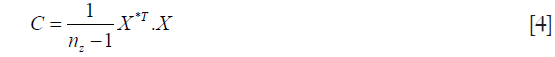
The covariance matrix C is then decomposed into the Eigen-components:

where λκ is the k-th Eigen value, and eχ is the k-th Eigen-vector. Since the assumption about the static and blood flow signals holds in most situations, Eigen-regression filter (18,19) is applied to the original signal by removing the first or two principal components (i.e., K =2 for  ) that represent the static signal:
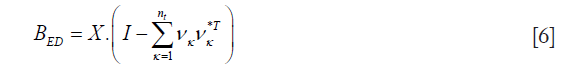
where B is the nz × nt blood flow signal matrix with added white noise. There are many other strategies which are proposed to adaptively determine the weighting coefficients for each principal component, but fix-rank filter will be our main focus due to its simplicity.
SVD
Another alternative to achieve PCA is the SVD, which can be applied directly onto our complex data matrix, X, without constructing an estimated covariance matrix, C, as in comparison to ED technique. SVD also has higher numerical accuracy, i.e. numerical precision by computing the quadratic term X*T, X, especially when the values of entries in our complex data matrix is discretely small.
In SVD technique, the data matrix, X, is decomposed into:
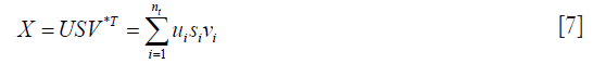
where U is left singular nx × nx unitary matrix, S is a diagonal nx × nt matrix of singular values, V is right singular nt × nt unitary matrix. Since the data matrix XC is usually large (nx >> nt) and we only interested in the sparse (random and uncorrelated) information. The computations of a subset (first K values) of the (nt) singular values are preferable as the computing time is significantly reduced.
The blood flow signal can be separated by rejecting the static and slow-moving signal:
SVD is similar to ED in theory and should give the exact same results when implemented with the same filtering strategy. More importantly, the work on SVD is motivated by its simplicity, numerical accuracy, and most importantly enabling further development of RPCA on OMAG.
RPCA
PCA is arguably the most widely used statistical tool for data analysis and dimensionality reduction. However, as PCA is sensitive to outliers, gross errors and corrupted observations (e.g., speckles, noise, and motion artifacts) can easily jeopardize the ability to separate the static tissue signal from the dynamic blood flow signal. Over the past decades, techniques classified as RPCA has been investigated to address this problem (23,24). RCPA works by recovering a low-rank matrix, L0 (static OCT signal), and a sparse matrix, S (dynamic blood flow OCT signal), from highly corrupted measurements, X = L0 + S (OCT complex dataset). There are many applications where the data can be modelled as low-rank and sparse components, such as video surveillance and face recognition (24). In medical imaging, robust principal component pursuit (RPCP, a variant of RPCA technique to be specific), has been adopted for magnetic resonance imaging and X-ray computed tomography since 2010s (25,26). This new method promises an improved visualization of dynamic signal and background suppression. However, at the time of writing, the applicability of RPCA in OCTA is still in question and has not yet been addressed in full.
In this paper, we implement a technique in RPCA, also called stable principal component pursuit (SPCP) (27), in separating the static structure and dynamic blood flow OCT signals. Amongst other RPCA techniques, SPCP requires less processing power whilst providing adequate dynamic blood-flow signal filter. In addition, this technique also seeks for an explicit noise component within the RPCA decomposition.
In OMAG, the low-rank and sparse matrix can be thought of as static structural and dynamic blood flow signals, respectively. The analysis starts with a given noisy-complex data matrix X. SPCP decompose X into a sum of low-rank matrix, L0, and a sparse matrix, S, with an added noise term, Z0:

The objective here is to recover the unknown matrix L0 and S, via a convex program:
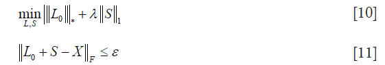
where ε represents the noise term and is assumed to be  , given that
  is the Frobenius norm of our noise term Z0; λ controls the weighting between static and blood flow signal;
  is the nuclear norm of L and
  is the 1-norm of S, calculated as:
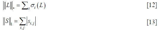
where  is the sum of singular values of L0 (L0 = USV*T), and
  is the sum of the absolute values of all entries in S. Static signal can be thought of as low-rank matrix, L, and blood flow signal can be thought of as sparse matrix, S.
In order to eliminate confusion in terminology, it should be made clear that author would use the term PCA (achieved by ED, SVD) and RPCA (achieved by SPCP) when discussing techniques in a broader sense.
Methods
In this study, PCA and RPCA are performed on the same sets of OCT complex data, which was acquired using a dedicated OCT system. The first set of OCT data was obtained by imaging a microfluidic-channel phantom. The second set of data was collected from human nail-fold tissue in vivo.
Microfluidic channel phantom
Scanning system and materials
SD-OCT system with broadband super-luminescent diode (LS2000C, Thorlabs Inc., Newton, NJ, USA) as the light source was used to capture the sets of imaging data from microfluidic channel phantom [details of the system description in (17)]. Briefly, the system had central wavelength 1,340 nm, and bandwidth of 110 nm, which provides approximately 7 µm of axial resolution in air. The lateral resolution of 7 µm was measured at the focus by using a 10× objective lens on the sample beam. The spectral interferograms between the beams from sample and reference arms were collected by a spectrometer based on a high-speed line-scan camera (1024-LDH2, Sensors Unlimited, Princeton, NJ, USA), providing 91.2 kHz A-line scan rate. The power of the sample beam was 3.5 mW, and the system had a sensitivity of 105 dB.
Scanning protocols were set to perform M-B scanning, with B-scan image showing the cross-section of the microfluidic channel inside the sample. The protocol anticipated the OCT beam at one A-scan position to acquire 50 repeated A-lines as one M-scan, then the beam moved across 200 positions, forming a full M-B scan of 2.8 mm × 1.4 mm (x by z, i.e., width by height). Raw interferometric spectrum was captured by camera, then the background signal was subtracted, followed by k-space linearization and then FFT to obtain complex OCT data (28). The final complex data matrix was in the form of 400×200×50 (nz × nx × nt) pixels, with spatial resolution of approximately 7 µm (axial) and 10 µm (lateral) and temporal resolution of 50 µs.
The microfluidic channel phantom consisted of a set of four perfused channels (5% intra-lipid solutions), which were embedded in a scattering background made of poly-dimethyl-siloxane (PDMS) mixed with titanium oxide (TiO2) powder. The cross-sections of the channels were rectangular in shape. There were four microfluidic channels with various sizes: 120 µm × 40 µm (R1), 60 µm × 40 µm (R2), 30 µm × 40 µm (R3), 15 µm × 40 µm (R4). The flow inside the channels were maintained by the external precision syringe pump (Harvard Apparatus PHD ULTRA, Massachusetts, USA) with programmable flow rate. Please see the detail of the phantom fabrication in (17).
Eigen/SVD and SPCP decomposition
Since Eigen and SVD decompositions yield similar results in most cases, the data is thus analyzed using ED algorithm in all following experiments. It is also important to distinguish the difference between strategy and technique in the context of OCT blood flow analysis. In this paper, strategy refers to different methods of organizing the complex data matrix before applying statistical analysis (i.e., Eigen, SVD, SPCP); and technique refers to different methods of statistical analysis. Although algorithm for each technique remains the same for most of our analysis, strategy does require adaptation upon the nature of the complex data matrix. For example, data from a still object can be arranged into Casorati matrix (one B-frame re-arranged into a vector, and each vector represent a repeated frame); whilst the same strategy (re-arranging data into Casorati matrix) would not work well on an in vivo sample where sampling volume is under constant motion. In fact, the term ‘motion artifact’ arises to describe the diminishing blood-flow signal to noise ratio (B-SNR) when data signals de-correlates between slow-time frames due to motion.
In this experiment, the strategy is to re-arrange our complex data matrix into Casorati matrix 80,000×50 (nzx × nt). For relatively stable object, this strategy helps improve the processing speed without compromising the image quality. The speed improvement is typically 5 to 10-fold faster than just comparing between pairs of frames on each A-line, depending on how many nt frames are analyzed. The flow image is revealed by removing the first two principal components, K =2, as in Eigen/SVD decomposition; and by choosing λ =0.007 [about 20 times the suggested value  (24)] and ε =0.12 in SPCP technique. The choice of λ is purely subjective, and was decided for the best contrast between the OCT dynamic blood flow and static structure. Examples of how varying λ parameter would affect the OCTA images are discussed in nailfold imaging in vivo.
Nail fold imaging in vivo
Scanning system and materials
In this experiment, the same SD-OCT system was employed for dynamic blood flow imaging. The imaging protocol was eight repeated B-scans for each of 400 y-direction scans, i.e., B-M scanning mode, producing a data matrix of 300×400×8×400 pixels (nz × nx × nt × ny).
Eigen/SVD and SPCP decomposition
Whilst scanning is performed on the sample under inevitable motion due to in vivo imaging nature, two major problems arise: (I) static signal becomes more dynamic between repeated frames; and thus (II) blood flow signal to noise ratio is significantly reduced, especially if the repeated-frame rate is less than a few hundred Hertz. For nail-fold experiments, the total number of repeated frames was eight, nt =8, and the repeated B-frame rate was 125 Hz. This imaging protocol gives an effective ensemble-frame (nt =8) rate of 15.6 Hz. Therefore, the choice of our imaging protocol was a compromise between the scanning range/resolution and the B-frame rate. For any given B-frame rate, a shorter scanning range can improve the lateral-scan density (i.e., more A-scans within one B-scan); and similarly, a longer scanning range with any given lateral-scan density would require a lower B-frame rate. In our experiment, 8 repeated B-frames with 125 Hz or higher frame rate is adequate for most biological sample, providing that the sample is moderately restrained on the scanning table.
ED/SVD analysis was performed on 300×400×8×400 (nz × nx × nt × ny) complex data matrix by decomposing the covariance of the B-M-frame Casorati matrix (nzx × nt =120,000×8 pixels) into 8 principal components, then removing the first two principal components (K =2) via Eigen-regression filter. The variance from the filtered data matrix was computed between the frames, i.e., var(BED) in slow-time, and the intensity of this variance vector (nz) was displayed in log scale. This process was repeated to form a filtered B-scan image (nz × nx), and finally a volume of dynamic blood flow (nz × nx × ny). This volume was then projected onto x-y plane, with color coded for depth, and intensity coded for the logarithmic variance value.
In RPCA, the data matrix input was the same as in ED analysis. The choice of lambda parameter was multiplied with a factor of 20 from the suggested value (24), i.e.,  , and ε =2e-2. This factor could vary between 10-200, depending on how much OCT dynamic blood flow signals one would like to retain. In general, higher value of this factor would result in only higher dynamic OCT signal being filtered in angiograms. The sparse (filtered) matrix was also post-processed for display, the procedure of which was the same as in the ED case.
In order to compare between PCA and RPCA, all of our resultant data matrices were normalized in log scale, using log1p function of MATLAB. The top-down, or x-y plane, projection was a maximum intensity projection with the depth (of pixel with maximum intensity) color-coded.
Results
Microfluidic chip phantom
Both SVD and ED produced similar results in separating the static and blood flow signal from the raw complex data (Figure 2). The rank (K =2) was chosen so that static signal was appropriately filtered out, but not to compromise the loss of information in flow signal. Figure 3 demonstrates the loss of information in flow signal (i.e., lower signal to noise ratio) when higher rank, K, was filtered out. In order to recover the flow signal, the filtered rank, K, needed to be as low as possible (i.e., as few principal components being filtered as possible).


On the other hand, SPCP controls the contributions of both static and blood flow signal via a weighting parameter lambda, λ. A higher value of λ would filter out more static and speckle signal, but with information loss in flow signal; whilst lower value of lambda would result in higher contribution of static and speckle signals. In addition, a higher value of the error term epsilon, ε, helps reduces the time for the convergence in the optimization problem. However, the information in flow signal (and partially speckle signal) is also lost at the expense of analysis time reduction.
The results are displayed in log scale and are presented in Figure 2. The data was further processed with semi-automatic segmentation (29) to calculate the signal to noise ratio among the three analyses (Table 2). The performance in processing time between ED and SVD was similar, while SPCP took longer to converge, depending on the precision of convergence in SPCP. In general, SPCP can achieve higher flow SNR in comparison to ED/SVD thanks to the ability to fine tune the weighting parameter λ. However, to achieve a detailed result, SPCP takes much longer time to converge and should be taken as a drawback, regarding performance quality-time cost.

Full table
Another important feature of SPCP is that we can control the amount of dynamic flow information through the weighting parameter lambda and fine-tune this parameter to our needs. This advantage is especially important when the number of repeated frames is small. For example, rank-filter in SVD (or Eigen-regression filter in ED) is a discrete number and might yield significantly different results when different rank is chosen. For example, when the number of repeated frame is small, nt =4, the result from K =2 filter would include too much speckles, whilst result from K =3 filter would lose too much flow information. This problem is discussed further in the results of nail-fold experiment, where the repeated frame is nt =8.
Nail-fold in vivo experiment
ED filter reveals adequate blood-flow SNR, but suffers from motion and tail-noise artifacts. Since the number of repeated frames in slow-time scan is small, the number of (filtered) principal components becomes important. The maximum number of ensembles in slow-time axis was 8 (nt =8), which constrained suitable Eigen-regression filter to either the first principal components (K =1) or first two principal components (K =2). Filtering third principal component in addition to the first two (K =3) would significantly degrade dynamic blood flow signals, whilst offering little benefits in static signals filtering. This argument is demonstrated in Figure 3 where dynamic flow SNR decreases with respect to a higher number of principal components (ranks) being filtered. All snapshots in Figure 3 are intensity presentations of microfluidic flow data in phantom experiments, displayed in log scale, and normalized between 0 and 1 in gray scale.
In addition to selecting the number of filtered principal components in ED/SVD analysis, choosing the number of frames in an ensemble is also important. The larger number of frames in one ensemble would yield higher blood flow SNR, providing that the tissue motion is not significant. A comparison between 8-frame ensemble and 5-frame ensemble, with the same filtered principal components, is shown in Figure 4.
The scanning protocol is also an important factor in ED analysis, especially the parameters of the repeated (slow-time) scan. A higher number of repeated scans and faster repeated scan rate would improve the blood flow SNR, assuming that the static signals amongst the scans are stationary. However, perfectly stationary sample rarely occurs and ‘motion artifacts’ are often introduced in ED/SVD analysis. The phenomenon of ‘motion artifacts’ can be seen as a significant reduced blood flow SNR in one particular filtered B-frame image. Equivalently, motion artifacts can be seen as higher intensity stripes across the projected x-y images (Figure 4). Motion artifacts are caused by decorrelation of static signals between certain number of frames, which skew our ED/SVD analysis. This sensitivity due to outliers (out-of-plane observation) is well known in ED/SVD (PCA) analysis (30). In order to improve image quality in ED/SVD analysis, the number of ensemble in slow-time axis (or number of repeated B-frames) should be as large as possible, but only up to certain limit that static signals start to de-correlates between the frames in the ensemble. This requirement dictates how scanning protocols is selected for optimal results in various cases. For example, sample under dynamic motion is typically scanned at 400 Hz with 8 repeated frames; whilst stable sample could be scanned at 100 Hz with 4 repeated frames.
Additionally, SPCP seems to be less affected by motion and tail-noise artifacts, whilst introducing speckles artifacts. In details, motion artifacts can be seen as horizontal stripes on the top-down (x-y plane) projection image from ED/SVD analysis, but the same motion artifacts are suppressed in SPCP analysis (Figure 5). On the same figure, tail-noise artifacts from ED/SVD analysis can be seen as strong vertical stripes below strong signals in B-frame images. The suppression of motion and tail-noise artifacts in SPCP is expected, as SPCP is not sensitive to outliers in comparison to ED/SVD (30). Speckle artifacts, however, seems to be enhanced under SPCP and manifest as a cloud of speckles on top of the flow signal (Figure 6) when suggested value of lambda,, is chosen. This ‘speckle cloud’ is reduced by tuning the weighting parameter, lambda, to a higher value. However, this ‘tune-up’ procedure comes with a loss in blood flow information, suggesting that ‘speckle cloud’ has some similarity to dynamic blood flow signal. Upon closer inspection, the ‘speckle cloud’ seems to have high degree of spatial connectivity (Figure 7). The dynamic signals, which form ‘speckle cloud’, also locates in stratum spinosum region (Figure 7—top right); and their patterns occasionally form loops with cavities of approximately 20–30 micrometers in size. Since the sizes of these loops are similar to the size of spinous cell and that their patterns resemble a honeycomb (31), it is possible that ‘speckle cloud’ represents the inter-cellular connection (desmosomes) of spinous cell. However, more investigations and evidence are needed to find a definitive answer to whether this ‘speckle cloud’ is indeed signals from the desmosomes of spinous cell.


Discussion
The raw OCT data holds most information about a sample of interests, including static structure and dynamic blood flow information. However, since our data is often large (typically 5 to 50 GB of memory) and not all information is required for diagnosis of certain disease. Therefore, raw data is usually processed and filtered to reveal the information of dynamic blood flow signal, which provides more clinical relevance about a particular disease. The reduction of information in our analysis achieves two things: (I) reduce the amount of information for further analysis; and (II) projecting our data onto new sets of bases which reveal most variance between frames (i.e., dynamic blood flow signal, speckles and noise). ED/SVD and SPCP analysis works on the same principal, where static and dynamic blood flow signals are filtered by comparing between the repeated frames within an ensemble.
ED/SVD, as one of the techniques in traditional PCA, constructs the rank k subspace approximation to the nt-dimension—nz observations that is optimal in a least-square sense (26). However, least-square techniques are not robust in a context where outlying measurements can arbitrarily skew the solution from the desired solution (24). A few examples are tail-noise (strong scatters) and motion artefacts (low coherence of static signal between frames in an ensemble). Both examples produce bright stripes across the filtered data matrix, which represents a significantly lower blood flow SNR, in comparison to other regions not being affected.
This paper revisits current PCA techniques, and implement SPCP to improve the complex blood flow analysis. SPCP decomposes the observation matrix X, an ensemble of repeated A-scan lines, into static (low-rank), dynamic blood flow (sparse) and noise. Since the observations are often corrupted by noise, motion, and highly scattered speckles, adding a noise term seems to be a natural choice. The resulting blood flow matrix from SPCP analysis shows less motion and tail-noise artefacts. While the examples illustrate benefits of SPCP in comparison to ED/SVD, the disadvantages of SPCP should also be taken into account in order to avoid unwanted results. Perhaps too sensitive to the changes in signal between the repeated frames, SPCP introduces significantly more speckles artifacts, which are not ‘true flow’. In the example of nail fold, this unwanted result resembles desmosomes of spinous cell, and is questionable to whether this observation could be useful additional information.
Conclusions
In summary, ED/SVD (or PCA) and SPCP separate dynamic blood flow from static structure by assuming that the static signals between the repeated frames is highly correlated. ED/SVD employ linear-regression filter and thus, is sensitive to outliers (tail-noise and motion artifacts). While SPCP is robust against outliers, this technique seems to enhance unwanted results albeit small in intensity. Lastly, RPCA (or SPCP in specific) is still computationally expensive, however, reader should keep in mind that RPCA is still under rapid development for efficiency and robustness at the time of writing.
Acknowledgements
Funding: This work was supported in part by grants from the National Heart, Lung, and Blood Institute (R01HL093140), the National Eye Institute (R01EY024158), Washington Research Foundation and an unrestricted fund from Research to Prevent Blindness. The funding organizations had no role in the design or conduct of this research.
Footnote
Conflicts of Interest: Dr. Wang discloses intellectual property owned by the Oregon Health and Science University and the University of Washington related to OCT angiography, and licensed to commercial entities, related to the technology and analysis methods described in parts of this manuscript. The other authors have no conflicts of interest to declare.
Ethical Statement: This study was conducted under a protocol approved by the University of Washington Institutional Review Board (No. 41841).
References
- Tarkin JM, Dweck MR, Evans NR, Takx RA, Brown AJ, Tawakol A, Fayad ZA, Rudd JH. Imaging Atherosclerosis. Circ Res 2016;118:750-69.
- De Backer D, Orbegozo Cortes D, Donadello K, Vincent JL. Pathophysiology of microcirculatory dysfunction and the pathogenesis of septic shock. Virulence 2014;5:73-9.
- Allen J, Howell K. Microvascular imaging: techniques and opportunities for clinical physiological measurements. Physiol Meas 2014;35:R91-141.
- Huang D, Swanson EA, Lin CP, Schuman JS, Stinson WG, Chang W, Hee MR, Flotte T, Gregory K, Puliafito CA, et al. Optical coherence tomography. Science 1991;254:1178-81.
- Tomlins PH, Wang RK. Theory, developments and applications of optical coherence tomography. J Phys D Appl Phys 2005;38:2519-35.
- Reif R, Wang RK. Label-free imaging of blood vessel morphology with capillary resolution using optical microangiography. Quant Imaging Med Surg 2012;2:207-12.
- Zhang A, Zhang Q, Chen CL, Wang RK. Methods and algorithms for optical coherence tomography-based angiography: a review and comparison. J Biomed Opt 2015;20:100901.
- Chen CL, Wang RK. Optical coherence tomography based angiography Biomed Opt Express 2017;8:1056-82. [Invited].
- Chen CL, Bojikian KD, Gupta D, Wen JC, Zhang Q, Xin C, Kono R, Mudumbai RC, Johnstone MA, Chen PP, Wang RK. Optic nerve head perfusion in normal eyes and eyes with glaucoma using optical coherence tomography-based microangiography. Quant Imaging Med Surg 2016;6:125-33.
- Kam J, Zhang Q, Lin J, Liu J, Wang RK, Rezaei K. Optical coherence tomography based microangiography findings in hydroxychloroquine toxicity. Quant Imaging Med Surg 2016;6:178-83.
- Kashani AH, Chen CL, Gahm JK, Zheng F, Richter GM, Rosenfeld PJ, Shi Y, Wang RK. Optical coherence tomography angiography: A comprehensive review of current methods and clinical applications. Prog Retin Eye Res 2017;60:66-100.
- An L, Qin J, Wang RK. Ultrahigh sensitive optical microangiography for in vivo imaging of microcirculations within human skin tissue beds. Opt Express 2010;18:8220-8.
- Wang RK, An L, Francis P, Wilson DJ. Depth-resolved imaging of capillary networks in retina and choroid using ultrahigh sensitive optical microangiography. Opt Lett 2010;35:1467-9.
- Wang RK, Jacques SL, Ma Z, Hurst S, Hanson SR, Gruber A. Three dimensional optical angiography. Opt Express 2007;15:4083-97.
- Reif R, Zhi Z, Dziennis S, Nuttall AL, Wang RK. Changes in cochlear blood flow in mice due to loud sound exposure measured with Doppler optical microangiography and laser Doppler flowmetry. Quant Imaging Med Surg 2013;3:235-42.
- Yousefi S, Qin J, Zhi Z, Wang RK. Uniform enhancement of optical micro-angiography images using Rayleigh contrast-limited adaptive histogram equalization. Quant Imaging Med Surg 2013;3:5-17.
- Wang RK, Zhang Q, Li Y, Song S. Optical coherence tomography angiography-based capillary velocimetry. J Biomed Opt 2017;22:66008.
- Zhang Q, Wang J, Wang RK. Highly efficient eigen decomposition based statistical optical microangiography. Quant Imaging Med Surg 2016;6:557-63.
- Yousefi S, Zhi Z, Wang RK. Eigendecomposition-based clutter filtering technique for optical micro-angiography. IEEE Trans Biomed Eng 2011;58.
- Sullivan TJ. Spectral Expansions. In: Sullivan TJ. editor. Introduction to Uncertainty Quantification. Cham: Springer International Publishing, 2015:223-49.
- Demené C, Deffieux T, Pernot M, Osmanski BF, Biran V, Gennisson JL, Sieu LA, Bergel A, Franqui S, Correas JM, Cohen I, Baud O, Tanter M. Spatiotemporal Clutter Filtering of Ultrafast Ultrasound Data Highly Increases Doppler and fUltrasound Sensitivity. IEEE Trans Med Imaging 2015;34:2271-85.
- Yu A, Lovstakken L. Eigen-based clutter filter design for ultrasound color flow imaging: a review. IEEE Trans Ultrason Ferroelectr Freq Control 2010;57:1096-111.
- Jolliffe IT, Cadima J. Principal component analysis: a review and recent developments. Philos Trans A Math Phys Eng Sci 2016;374:20150202.
- Candès EJ, Li X, Ma Y, Wright J. Robust principal component analysis? J ACM 2011;58:11.
- Otazo R, Candès E, Sodickson DK. Low-rank plus sparse matrix decomposition for accelerated dynamic MRI with separation of background and dynamic components. Magn Reson Med 2015;73:1125-36.
- Gao H, Yu H, Osher S, Wang G. Multi-energy CT based on a prior rank, intensity and sparsity model (PRISM). Inverse Probl 2011;27:115012.
- Zhou Z, Li X, Wright J, Candès E, Ma Y. Stable principal component pursuit. In: IEEE International Symposium on Information Theory Proceedings (ISIT 2010), 2010:1518-22.
- Wang RK, Ma Z. A practical approach to eliminate autocorrelation artefacts for volume-rate spectral domain optical coherence tomography. Phys Med Biol 2006;51:3231-9.
- Yin X, Chao JR, Wang RK. User-guided segmentation for volumetric retinal optical coherence tomography images. J Biomed Opt 2014;19:086020.
- De la Torre F, Black MJ. Robust principal component analysis for computer vision. Proceedings Eighth IEEE International Conference on Computer Vision. ICCV 2001.
- Meyer LE, Otberg N, Sterry W, Lademann J. In vivo confocal scanning laser microscopy: comparison of the reflectance and fluorescence mode by imaging human skin. J Biomed Opt 2006;11:044012.

