
A low-cost pathological image digitalization method based on 5 times magnification scanning
Introduction
In pathological examinations, technicians make glass slides of human tissue, such as routine hematoxylin and eosin (HE) (1), frozen sections (2,3), and special staining (4). The pathologist magnifies the slides with a microscope to diagnose the disease. In recent years, the digitalization of pathological slides has begun to be promoted because of convenient storage, network transmission, and effective computer-aided diagnosis (5-7).
A high-resolution (HR) scanner with 20 times magnification (20×) or even a 40× lens is used to scan the glass slide, and the whole slide image (WSI) is obtained (8). Because of multiple magnifications of image, one WSI contains up to 50,000×50,000 pixels (9), and the file size per 40× WSI may range from 1 gigabyte (GB) to 5 GB, depending on the size of the specimen in the slide (10), which significantly increases the storage costs and takes a few minutes for network exchange (11). The development of digital pathology requires the preservation of a large number of WSIs for a long time. Taking China as an example, there are as many as 50 million new pathological examinations every year, which requires 50,000,000 to 250,000,000 GB storage capacity. Moreover, the HR scanning of each WSI needs a few minutes or more (12), so the digitization of the WSIs requires more than 200 years of scanning time. In addition, because the depth of field of the HR lens is very small, the tissue on the slide must be very flat or parts of the WSI may be blurred (13). Therefore, the HR digitalization of pathological glass slides is inefficient and costly.
We assume that low-resolution (LR) scanning, such as 5× magnification, can provide an alternative strategy. Compared with 40× scanning, the speed of 5× scanning increases by 64 times, and the size of WSI reduces to 1/64. Second, the depth of field of the LR lens is larger, which could reduce requirements about the flatness of human tissues. However, the 5× images have lost many details for diagnosis, so a method must be proposed to restore the missing details and generate a series of HR images from 5× images.
The conventional methods of obtaining HR images from LR images are algorithms such as bilinear interpolation and bicubic interpolation (14). However, it is difficult for them to recover the lost details. Recently, to obtain high-quality images from LR images, superresolution (SR) methods based on deep learning have been widely studied in natural images. There are many excellent SR algorithms, such as deep recursive residual networks (DRRNs) (15), SR generative adversarial networks (SRGANs) (16), progressive generative adversarial networks (P-GANs) (17), and multiscale information cross-fusion networks (MSICFs) (18). SR methods are also used in medical images such as magnetic resonance (19,20), computer tomography (21), and ultrasound images (22). For example, the SR convolutional neural network (SRCNN) is used for computer tomography images (23), and the pathological SR model is used for cytopathological images (24).
Although SR methods have been successfully applied in many domains, pathological images are different from natural and other medical images. There are a large number of cells and rich microtissue structures in them, but general SR methods pay attention to the larger image texture and structure. Moreover, the maximum magnification of almost all SR methods is 4 times (25), but the magnification of the pathological image is up to 8 times, e.g., from 5× to 40×. For the convenience of diagnosis, a series of HR images should be continuously obtained from 5× images; however, the magnification of almost all SR methods is fixed. We propose a multiscale SR method (MSR), which continuously generates 10×, 20×, and 40× SR images from 5× images. The highlights of the proposed method are as follows:
The size of the 5× scanned image is small enough, approximately 15 Megabytes (MB), and only one-64th of the image file is scanned by 40×. The presented method can generate 10×, 20×, and 40× SR images simultaneously. The optimization is applied on three resolutions, and the generated images are of realistic and rich details, better than the existing methods.
The differences between generated and real images are evaluated based on the pathological diagnosis of 10 types of human body systems, which shows the potential for clinical applications. Therefore, MSR is promising as a low-cost method for pathological digitalization.
We present the following article in accordance with the MDAR checklist (available at https://qims.amegroups.com/article/view/10.21037/qims-21-749/rc).
Methods
The study was conducted in accordance with the Declaration of Helsinki (as revised in 2013). The study was approved by the Institutional Review Board of Xiangya Hospital, Central South University (No. 2019030596), and individual consent for this retrospective analysis was waived.
Dataset collection
Pathological glass slides were obtained from Xiang-ya Hospital of Central South University, which is one of the most famous hospitals in China. The technicians randomly selected 200 whole slides, including 10 types of human body systems, from the pathological archive of the hospital (Table S1). Slides from 10 types of human body systems were selected to ensure the generalization of the dataset because the pathological structures of different systems are different. The number of whole slides of each human body system was set to 20, and the WSIs of some typical diseases were randomly selected by technicians using the pathological archive search tool. The slides were then scanned using a KF-PRO-005 digital pathology scanner (KFBIO company, Ningbo City, China) to obtain WSIs at 40× magnification. After WSIs were obtained, the technicians no longer participated in the follow-up studies.
Dataset review
Two pathologists with “associate chief physician” titles and at least 10 years in the clinic reviewed the image quality of WSIs to ensure that the WSIs were suitable for pathological diagnosis. If the image quality of WSI was too poor to be suitable for diagnosis, it was excluded. They then independently reviewed the pathological tissue structures of WSIs for the diagnosis of diseases. If a consensus was reached, the WSI was included. No WSI was excluded due to image quality or inconsistent diagnosis. Finally, they discussed selecting two nonoverlapping regions of interest (ROIs) from each WSI for subsequent medical testing. The two ROIs were considered to include sufficient information on disease diagnosis. After reviewing WSIs, the two pathologists would no longer participate in follow-up studies.
Dataset division and preprocessing
The WSIs were randomly divided into training, testing, and extended medical testing sets, as detailed in Figure 1. The training set consists of 80 WSIs, which come from 10 types of human body systems, and each system has 8 WSIs. The testing and medical testing sets consist of 20 and 100 WSIs, respectively. Because the size of one WSI is too large to be inputted into the convolutional neural network, the 1,000 nonoverlapping images (tiles or patches) from every WSI in the training and testing sets are randomly taken out, and the size of every image is 1,024×1,024 pixels (40×). There are a total of 100,000 images in the training and testing sets. Among the 100 WSIs of the medical testing set, two ROIs of each WSI, selected by the two pathologists mentioned above, are used for medical evaluation.
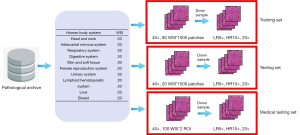
Because the pathological scanner has only two lenses, 20× and 40×, it is impossible to directly obtain LR images. To obtain LR images from the 40× images, the bicubic interpolation algorithm is used, where 3 continuous downsamples from each 40× image are used to obtain LR images of 20×, 10×, and 5× (26,27), which are 512×512, 256×256, and 128×128 pixels, respectively. Therefore, the 5×–20× images in the training and testing sets are obtained, which are treated as the real LR images. Meanwhile, the size of each pixel in the 40× image is 0.25 micrometers (KFBIO scanner by KFBIO company, Ningbo City, China), while the pixel sizes of 20×, 10×, and 5× images are 0.5, 1, and 2 mm, respectively.
The minimum dataset can be found at https://doi.org/10.6084/m9.figshare.15173634. The whole dataset can be obtained by contacting the author for research but cannot be used for commercial purposes.
Network architecture
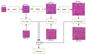
The proposed network comprises three superresolution blocks (SBRs), and each SRB can magnify the input image by 2 times. Therefore, by combining three SRBs, the network can magnify the input image by 2 times, 4 times, and 8 times. The 5× LR image is inputted into the network, and the 10×, 20×, and 40× SR images are continuously generated by the three SRBs, as shown in Figure 2. The generated images are compared with real images at three resolutions, and the pixel differences (generator loss), feature differences (perceptual loss), and image differences (discriminator loss) are weighted together to guide the training of the network.
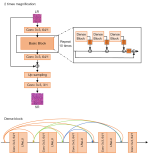
The structures of these SRBs are the same, as shown in Figure 3, where the input LR image is first convolved by 64 kernels with a size of 3×3, and the 10 repeated basic blocks are concatenated to predict the details in the SR image. The predicted details are mixed by a convolutional layer and then added to the input LR image. The sum of predicted and original details is upsampled, which is performed by a subpixel layer, where four convolution kernels are learned to increase the number of channels by four times, and the channels are reshaped to three for two upsamplings. Meanwhile, every basic block includes three dense blocks, where five dense convolutional layers are concatenated to find multiscale features from the LR image to reconstruct the lost details.
The loss functions, including the generator, perceptual, and discriminator losses, are based on three levels: pixel, feature, and whole image. The generator loss compares the differences of the pixels one by one of the generated images and real images and is defined as the mean absolute error.
where Xj is the magnification and m is the pixel number in the image. The SR is the generated image, and HR is the real image.
The high-level representations of generated SR images and real HR images are extracted, where a network of 19 layers from the Visual Geometry Group (VGG19) (28) is selected as the extractor because of its excellent performance on representation learning. The middle-level (layer 5) and high-level (layer 9) representations are compared here for the perceptual loss of the generated image and real image, defined as Eq. [2].
where Xj=10×,20×,40×, the MSE is the mean square error function, and ϕ is the extractor of VGG19.
To make better generated images that have a high degree of authenticity, the discriminator network is used to identify the true or false values of the real image and the generated image. Because the discriminator network will be trained with the generator, we only use one discriminator to compare the authenticity of the images with the maximum 40× magnification to reduce the training cost. Generally, the greater the magnification is, the more likely the generated image is to be distorted. Therefore, if the quality of the 40× image is good, 20× and 10× should also be good. The discriminator loss is defined as Eq. [3].
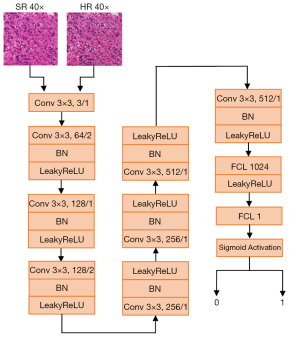
where D is the discriminator network. Because there are so many details in 40× pathological images, a very deep discriminator network is used, where there are seven convolutional modules and two fully connected layers. Every convolutional module includes some convolution layers with 64–512 convolutional kernels of 3×3 size, and the stride size is 1–2. The sigmoid function is connected to the end, outputting True [1] and False [0], as shown in Figure 4.
The two or three losses at each magnification are added and then weighted together for the total loss function.
where is the sum of generator, perceptual, and discriminator losses at magnification and is the weighted value.
Network training
The proposed network is implemented using the TensorFlow framework (version 1.15.0) (29) and trained on a server consisting of two graphics processing units (GPUs) of Tesla V100 32 GB (NVIDIA company, Santa Clara, California, USA). The pretrained model of VGG19 is downloaded from the model zoo of TensorFlow and remains fixed during training. The generator and discriminator are initialized randomly and trained alternately. The source code can be found: http://github.com/CSU-BME/pathology_MSR.
Ten percent of the images in the training set (8 WSIs, 8,000 images) are used as the validation set for hyperparameter selection. Different parameter values were tried, such as the optimizer (SGD, Adadelta, Adam), the initial learning rate (0.0005, 0.0004, 0.0001), and the batch size [2, 4, 6]. The optimal parameters with the best performance on the validation set were selected. The hyperparameters are listed in Table 1. The Adam optimizer is selected because of its good performance. The initial learning rate is 0.0004 and decays exponentially, where the rate is reduced by 0.5 times every 30 epochs. The total number of training epochs was 120, and 500 steps were performed every epoch. The batch size is fixed to 2, considering the GPU memory, patch size, and training costs. The 50 smaller patches with a size of 64×64 pixels are randomly selected from the input LR 128×128 image, and the small patches whose standard deviations are larger than the flatness value are kept and then input to the proposed network for training. The flatness is the parameter controlling the complexity of the input patches, and only the patches with complex details should be used as the training data. The flatness increases 0.01 from 0 every 5 epochs, but not more than 0.15. The weights of the three losses are determined after hyperparameter selection, where the weight of the generator loss is 0.06, perceptual loss 0.083, and discriminator loss 0.04.
Table 1
| Hyperparameters | Value |
|---|---|
| Epochs | 120 |
| Steps per epoch | 500 |
| Batch size | 2 |
| Learning rate | 0.0004 |
| Decay factor | 0.5 |
| Decay frequency | 30 |
| Min flatness | 0 |
| Max flatness | 0.15 |
| Increase factor | 0.01 |
| Increase frequency | 5 |
| Generator loss weight | 0.06 |
| Perceptual loss weight | 0.083 |
| Discriminator loss weight | 0.04 |
Experiment settings for quantitative comparison
The quantitative experiments are described here, and the 10×, 20×, and 40× SR images are generated from 5× images in the testing set by the proposed MSR method. While the 5× image is converted to 10×–40× images, the numbers of pixels are the same as the real 10×–40× images. Two quantitative indices are computed to evaluate the generation quality. The first is peak-signal-to-noise-ratios (PSNR), which is defined as the pixel-by-pixel similarity between two images (30). Its definition is as follows.
The mean square error (MSE) represents the difference in pixel-by-pixel value between two images, which is defined as Eq. 6.
where SR and Real indicate the generated image and real image, respectively. (i, j) are the coordinates of one pixel on the image, and M and N represent the width and height, in pixels, of the image, respectively. The image intensity ranges from 0 to 255, and the unit of PSNR is decibels (dB). From Eqs. [5,6], larger values of PSNR would indicate more similarity or less difference.
The second is the structural similarity (SSIM) index, which is defined as the similarity in human vision between two images (31). The definition is shown as follows:
where x,y are two images; μx and μy represent the mean brightness of the images x,y; and σx, σy, and σxy indicate the two variances and covariance, respectively. C1and C2 are the two known constants. Larger values of SSIM would indicate more similarity or less difference between the two images x,y.
To compare our model and other recent SR models, such as deep back-projection networks (DBPN) (32), efficient sub-pixel convolutional neural network (ESPCN) (33), enhanced deep superresolution network (EDSR) (34), multiscale deep superresolution system (MDSR) (34), and residual dense network (RDN) (34), the existing models are retrained and retested in our training and testing sets. Because these models support only a fixed magnification, three versions with 2 times, 4 times, and 8 times magnification of each model are trained and tested, for example, DBPN-10×, DBPN-20×, and DBPN-40×, which, respectively realize the generation of 10×, 20×, and 40× images from 5× images in the testing set. Similarly, after the PSNR and SSIM of the 10×, 20×, and 40× images generated by each model and the real 10×, 20×, and 40× images in the testing set are computed, all PSNRs and SSIMs are averaged at different resolutions. The codes of these models are downloaded from the links given in their published papers and then retrained at 2 times, 4 times, and 8 times magnification according to the provided hyperparameters in the codes. The RDN code produced some errors when magnifying the 5× image by 8 times (34), and the author of the RDN model did not give a solution, so the PSNR and SSIM of RDN at 40× images cannot be provided. Two conventional digital zoom methods, BILINEAR (bilinear interpolation) and BICUBIC (bicubic interpolation), are also compared with our model.
Experiment setting for medical diagnosis
Another 100 40× WSIs in the medical testing set were used to evaluate the pathological diagnosis by pathologists, as shown in Figure 5. Two nonoverlapping ROIs of every WSI were defined as HR ROI-1 and ROI-2, which were selected by the two pathologists mentioned in the dataset review subsection. The two ROIs from the same WSI are paired, and a total of 100 paired ROIs are obtained. We invited six highly experienced pathologists (A-F) who had all been in pathological clinics for at least 10 years to participate in this medical evaluation. None of them had access to the images before this experiment.
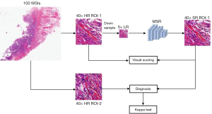
The reason why a preselected ROI is diagnosed is to exclude some influencing factors. When we compare the diagnostic difference between real images and generated images, there are three factors to consider: the difficulty of the disease, the pathologist’s diagnostic ability, and the difference in images. Among them, the first two differences must be ruled out first, and then the difference of diagnoses can show the difference between the two images. Therefore, we selected a pair of ROIs related to the disease from a WSI. Because these two ROIs come from the same patient, the same doctor diagnoses the same patient twice, so the two factors of the patient and the doctor’s ability will not affect the results. Therefore, the significant difference based on the ROI is only related to the image quality. In contrast, if the doctor is asked to see two different WSIs, one is real and the other is generated, then the differences of the patient and the doctor’s ability are included. In future diagnosis based on the newly scanned 5× images, we will start with 5× WSI and generate 10×, 20×, and 40× WSI by the presented SR model. The HR ROI-1 is downsampled to 5× LR and then input into the presented method (MSR) to generate the SR ROI-1. Because each pair of HR ROI-1 and SR ROI-1 comes from the same WSI of the same patient, pathologists should make the same diagnosis, regardless of the diagnostic ability of pathologists.
Results
The comparison of quantitative comparison
The 10×–40× SR images are generated from 20,000 5× images in the testing set and compared with real 10-40× HR images. The PSNR and SSIM distributions of our model, five SR models (DBPN, ESPCN, EDSR, MDSR, RND), and two conventional digital zoom methods (BILINEAR, BICUBIC) at different resolutions are shown in Figure 6. Additionally, the PSNR and SSIM of each body system are listed in Table S2. The average PSNR with 0.95 confidence interval of our method on 10×, 20×, and 40× are 24.167±3.734 dB, 22.272±4.272 dB, and 20.436±3.845 dB, respectively, and the average with 0.95 confidence interval are 0.845±0.089, 0.680±0.150, and 0.559±0.179.
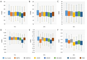
From Figure 6, it can be seen that the SSIM and PSNR on the 10× images of all methods are the highest, which means that the images generated by 2 times magnification are the closest to the real images, and the image quality is the highest. Because 40× images are downsampled to 5× images and most details are lost, the quality of the generated 40× images is relatively poor. In contrast, our method has a higher mean PSNR and SSIM than the other methods at 10×, 20×, and 40× generated images, which shows that our method has a better restoration of image details (P value <0.05).
The comparison of visual inspections
Although the mean PSNR and SSIM can evaluate the similarity in signal and vision between the generated images and the real images, they are still far from human visual perception. In Figure 7, the real HR 10×, 20×, and 40× images are displayed in the left column, in which the ROIs are drawn by the green bounding box. The 10×, 20×, and 40× images generated from 5× ROIs by our model, the other SR models and two conventional digital zoom methods, and real ROI images are shown in the right column. By visually inspecting the generated images, it can be found that for 10×, all the generated images are of high quality and the image details are quite realistic.
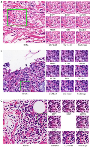
Additionally, it is evident that the 20× images from our model are relatively close to the real image, but other methods have different degrees of distortion. Moreover, the 40× images generated by other models appear blurred, while our model can preserve important image structures. It is worth noting that from 5× to 40×, some backgrounds are too small to be completely restored, which is consistent with the PSNR and SSIM.
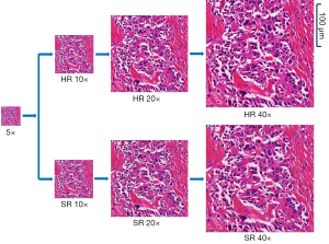
The images generated by our method and real images of one typical sample are shown in Figure 8, which shows that the visual perception of generated and real images is very similar. Pixel-sized scale is also shown on the 40× image.
Visual comparison for medical evaluations
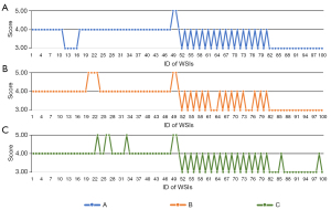
The first comparison is the visual scoring of HR ROI-1 and SR ROI-1. Three pathologists (A-C) carefully observed the two images and then gave a score on the diagnostic consistency of the two ROI images. The scoring rules are shown in Table 2, where the visual scoring results are set to five different levels denoted by 1–5 to represent the quality of generated images. A more significant value implies better quality. When pathologists compare any pair of real and generated ROIs, if they think that important information for a correct diagnosis is retained in the generated ROI, the score is 3. For example, the features of cancer cells in cancer images are completely preserved. A total of 100 pairs of HR ROI-1 and SR ROI-1 were scored by pathologists A-C. The distributions of visual scorings from three pathologists are shown in Figure 9, and the average score on each body system is shown in Table S3. Figure 9 shows that the three pathologists agreed that all generated ROIs retained diagnostic features, so the ROIs scored at least 3. Regarding the closeness of the generated ROI to the real ROI, pathologists have inconsistent scores of 4–5, which may be due to differences in their subjective perceptions of the restoration of the generated image. The average visual scorings with 0.95 confidence intervals from pathologists A, B, and C were 3.630±1.024, 3.700±1.126, and 3.740±1.095, respectively, indicating that the pathologists believe that there is no visual difference in diagnosis between the generated image and the real image or that the visual difference will not affect the diagnosis. The P value of analysis of variance was 0.367, meaning that the scores of the three pathologists were not significantly different.
Table 2
| Scores | Descriptions |
|---|---|
| 5 | The differences between the generated and real images are so small that they are almost invisible |
| 4 | There is a slight difference, but it does not affect the diagnosis |
| 3 | There is a certain difference, but it does not affect the diagnosis |
| 2 | There are noticeable differences, which may affect the diagnosis |
| 1 | The difference is large enough not to be used for diagnosis |
Diagnosis comparison for medical evaluations
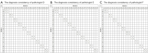
To obtain quantitative comparisons of the generated image and the real image diagnosis, the covariates of the difference between the diagnosis difficulty of the sample and the diagnosis ability of the pathologists should be removed. Therefore, the 100 paired SR ROI-1 and HR ROI-2 are randomly shuffled. Except for the human body system from which the images come, other information, including the WSIs to which the ROIs belong, has been eliminated. Another three pathologists (D-F) blindly reviewed the SR ROI-1 and HR ROI-2 independently and made diagnoses for every ROI.
The diagnosis comparison is shown in Figure 10, where the ROIs of the generated images were misdiagnosed twice and the ROIs of the real images were misdiagnosed once. Compared to the total number of ROIs, the error ratio of the generated and real images is very close. The Kappa test shows that KD (K value of pathologist D) about the 100 paired SR ROI-1 and HR ROI-2 from pathologist D is 0.990, KE from pathologist E is 1.000, KF from pathologist F is 0.980, showing no significant difference in the diagnosis of three pathologists based on the generated images and the real images.
Generation time and diagnosis time
A 5× ROI containing 128×128 pixels can be converted to 10×, 20×, and 40× ROIs in 200 ms using a graphics processing unit of Tesla V100. If the server has 4 GPUs and the WSI has 4,000 ROIs with human tissue, the conversion from a 5× WSI to 10×–40× WSI would take 3–4 min.
The average time with 0.95 confidence intervals while diagnosing one generated ROI or one real ROI was compared by a two-sided paired T test. Pathologist A: 5.849±2.200 vs. 5.951±2.349 s, P value =0.534; pathologist B: 6.497±2.649 vs. 6.269±2.944 s, P value =0.285; pathologist C: 7.147±3.691 vs. 6.893±2.398 s, P value =0.248. There was no significant difference in the diagnosis time between the generated image and the real image.
Discussion
Pathological slides are not conducive to preservation and are inconvenient to search and exchange. With the advent of HR scanners, pathological images from glass slides have been applied in modern pathology. The glass slides are scanned into digital WSIs, which can be conveniently stored and transmitted over the network for remote diagnosis. Because there are many microscopic cells and tissues in pathological slides, HR scanning is necessary to retain these image details. However, the file size of HR scanning is too large, which severely affects the acceptance of digital pathology because of the slow scanning and data exchange and huge storage costs.
We design an alternative strategy for LR scanning, where the 5× images are only approximately 15 MB, which is promising to solve the storage and exchange problems of pathological images. However, LR images, such as 5× images, only show large-scale structural information of human tissue. In fact, pathologists first observe LR images on a large scale and then use a larger magnification to observe the cells on a small scale. In other words, 40× image diagnosis and 5× image diagnosis are based on the information at different scales. The 5× images cannot support a complete pathological diagnosis because of the lack of small-scale information provided by 40× images.
If the structure is larger than 2 microns (one-pixel size in the 5× image), it can be recovered by SR. It is worth noting that structures smaller than 2 microns may be lost, or they cannot be fully restored based on adjacent pixels. The smallest structure concerned in pathological diagnosis is the nucleus of small lymphocytes, whose diameter is approximately 7 microns (35). The size of each pixel in the 40× image is 0.25 microns, so the nucleus of small lymphocytes includes 28×28 pixels. In the 5× image, the nucleus would include 3.5×3.5 pixels. Therefore, the smallest structure is present on the 5× image and should be restored from the 5× image to the 40× image by a good SR method.
Although the existing SR models have been widely used in natural and medical images, the main problem is fixed magnification, and the magnification is not more than 4 times. According to the needs of pathological diagnosis, the SR method must be magnified continuously, and the maximum magnification can reach 8 times. The proposed method meets the above requirements and can continuously generate 10×, 20×, and 40× images.
We performed paired T tests on SSIM and PSNR between our method and existing methods. PSNR is an index for evaluating the similarity of pixel-by-pixel values of two images, and no image structure, such as edge, region, and texture, is considered. A large PSNR value means that the pixel-by-pixel values of two images are close, but it does not mean that the human visual perceptions of two images are close. SSIM can compare the similarity of image structures; it is closer than PSNR but still different from human perception. In all experiments, the PSNR and SSIM of our method are higher than those of other methods.
Visual comparison is more effective in illustrating the advantages of our method, which is significantly better than those of the existing methods, especially the restoration of cell structure and clusters related to pathological diagnosis. However, it is worth noting that the PSNR and SSIM of all methods are lower than those of the natural images. Although our method can restore local details very well, the color of the generated image is slightly changed. This may be because the method pays attention to microstructures such as cells in the pathological image but not macrostructures such as the color and background of the image. The PSNR and SSIM mainly consider the differences in macrostructures, so the two indicators are not too high.
Because the existing SR models have only fixed magnifications, we trained three versions, i.e., the generations of 5×–10×, 5×–20×, 5×–40×. In theory, a model that considers a single magnification ratio should perform better than a model that generates multiple magnification ratios simultaneously because the learning task is easier. However, our method has achieved better results than those in quantitative evaluation and visual comparison experiments. The possible reason is that the image generated by our method is optimized with the real image at multiple resolutions/magnifications, but other methods only consider the optimization at a single magnification.
For application in pathological domains, whether the generated image can replace the real image, the most important factor is whether it changes the diagnosis result. Therefore, medical confirmation is more important. In the visual assessment, the pathologists believed that although there were visual differences between the generated image and the real image, the information required for diagnosis was complete.
Our clinical evaluation first chose the most important task of pathological diagnosis for cancer, including multiple cancers involving multiple organ systems. In addition, some inflammation and other benign lesions, such as hippocampal sclerosis, endometrial polyps, renal medullary lipoma, and kidney atrophy, are also included. Because the pathological diagnosis is based on human tissue structure and cells on the image, the process for cancer and other diseases is similar. If SR can provide the information of cells and human tissue structure needed for these diseases, we have reason to believe that the information needed for other disease diagnoses should also be generated. The blind diagnosis from 10 body systems confirmed that there was no significant difference between the diagnosis of generated images and real images in the medical testing set.
The development of digital pathology requires the preservation of a large number of whole slide images for a long time. Whether these images are 5× or 40× is related to storage capacity and copying or network transmission. Our research suggests permanently keeping 5× images instead of 40× images to reduce storage and transmission costs. The practical application of pathological images can be roughly divided into two common scenarios, among which the images to be generated are well known. First, for new patients in clinical practice, we can generate 40× images from new scanned 5× images in advance for pathologists to diagnose. After diagnosis, the 40× images are then deleted. Second, for scientific research issues, researchers have designed clear experimental settings, looking for suitable slides (5× images) from pathological archives, quickly transmitting the 5× images to the local server via the network, and then generating 40× images for research. When the image to be generated cannot be known in advance, although this is not common, it is a wonderful alternative that generates in real-time the 40× region of interest that the pathologist is observing because the generation time of a region is only approximately 200 ms.
Quantitative and visual experiments have confirmed the excellent image quality generated by the proposed method, and medical experiments on some specific diseases preliminarily confirmed that the generated images have the potential for clinical pathological diagnosis. The main limitation of this study is that there were not enough types of diseases in the test set. However, it shows the possibility of LR digitization, and it is worthwhile to further evaluate its feasibility on a wide range of datasets in further work.
Conclusions
Digital pathology can easily store and exchange WSIs, but the HR scan will produce large image files, high storage costs, and slow network transmission. The proposed multiscale method based on LR scanning can generate SR images with sufficient information for pathological diagnosis. The low-cost digital method was first proposed for pathology, showing potential for clinical application. In future work, on a large-scale image dataset, the diagnostic difference between the generated and real images should be further evaluated.
Acknowledgments
Funding: This work was supported by the Emergency Management Science and Technology Project of Hunan Province (#2020YJ004, #2021-QYC-10050-26366 to G Yu).
Footnote
Reporting Checklist: The authors have completed the MDAR checklist. Available at https://qims.amegroups.com/article/view/10.21037/qims-21-749/rc
Conflicts of Interest: All authors have completed the ICMJE uniform disclosure form (available at https://qims.amegroups.com/article/view/10.21037/qims-21-749/coif). The authors have no conflicts of interest to declare.
Ethical Statement: The authors are accountable for all aspects of the work in ensuring that questions related to the accuracy or integrity of any part of the work are appropriately investigated and resolved. The study was conducted in accordance with the Declaration of Helsinki (as revised in 2013). The study was approved by the Institutional Review Board of Xiangya Hospital, Central South University (No. 2019030596), and individual consent for this retrospective analysis was waived.
Open Access Statement: This is an Open Access article distributed in accordance with the Creative Commons Attribution-NonCommercial-NoDerivs 4.0 International License (CC BY-NC-ND 4.0), which permits the non-commercial replication and distribution of the article with the strict proviso that no changes or edits are made and the original work is properly cited (including links to both the formal publication through the relevant DOI and the license). See: https://creativecommons.org/licenses/by-nc-nd/4.0/.
References
- Wittekind D. Traditional staining for routine diagnostic pathology including the role of tannic acid. 1. Value and limitations of the hematoxylin-eosin stain. Biotech Histochem 2003;78:261-70. [Crossref] [PubMed]
- Arcega RS, Woo JS, Xu H. Performing and Cutting Frozen Sections. Methods Mol Biol 2019;1897:279-88. [Crossref] [PubMed]
- Švajdler M, Švajdler P. Frozen section: history, indications, contraindications and quality assurance. Cesk Patol Summer;54:58-62.
- Alturkistani HA, Tashkandi FM, Mohammedsaleh ZM. Histological Stains: A Literature Review and Case Study. Glob J Health Sci 2015;8:72-9. [Crossref] [PubMed]
- Niazi MKK, Parwani AV, Gurcan MN. Digital pathology and artificial intelligence. Lancet Oncol 2019;20:e253-61. [Crossref] [PubMed]
- Pallua JD, Brunner A, Zelger B, Schirmer M, Haybaeck J. The future of pathology is digital. Pathol Res Pract 2020;216:153040. [Crossref] [PubMed]
- Bueno G, Fernández-Carrobles MM, Deniz O, García-Rojo M. New Trends of Emerging Technologies in Digital Pathology. Pathobiology 2016;83:61-9. [Crossref] [PubMed]
- Aeffner F, Adissu HA, Boyle MC, Cardiff RD, Hagendorn E, Hoenerhoff MJ, Klopfleisch R, Newbigging S, Schaudien D, Turner O, Wilson K. Digital Microscopy, Image Analysis, and Virtual Slide Repository. ILAR J 2018;59:66-79. [Crossref] [PubMed]
- Tizhoosh HR, Pantanowitz L. Artificial Intelligence and Digital Pathology: Challenges and Opportunities. J Pathol Inform 2018;9:38. [Crossref] [PubMed]
- Hanna MG, Reuter VE, Hameed MR, Tan LK, Chiang S, Sigel C, Hollmann T, Giri D, Samboy J, Moradel C, Rosado A, Otilano JR 3rd, England C, Corsale L, Stamelos E, Yagi Y, Schüffler PJ, Fuchs T, Klimstra DS, Sirintrapun SJ. Whole slide imaging equivalency and efficiency study: experience at a large academic center. Mod Pathol 2019;32:916-28. [Crossref] [PubMed]
- Mukherjee L, Bui HD, Keikhosravi A, Loeffler A, Eliceiri K. Super-resolution recurrent convolutional neural networks for learning with multi-resolution whole slide images. J Biomed Opt 2019;24:1-15. [Crossref] [PubMed]
- Neil DA, Demetris AJ. Digital pathology services in acute surgical situations. Br J Surg 2014;101:1185-6. [Crossref] [PubMed]
- Liu S, Hua H. Extended depth-of-field microscopic imaging with a variable focus microscope objective. Opt Express 2011;19:353-62. [Crossref] [PubMed]
- Xia P, Tahara T, Kakue T, Awatsuji Y, Nishio K, Ura S, Kubota T, Matoba O. Performance comparison of bilinear interpolation, bicubic interpolation, and B-spline interpolation in parallel phase-shifting digital holography. Opt Rev 2013;20:193-7. [Crossref]
- Ying T, Jian Y, Liu X. Image Super-Resolution via Deep Recursive Residual Network. IEEE Conference on Computer Vision & Pattern Recognition, IEEE Computer Society, 2017:2790-8.
- Wu Y, Yang F, Huang J, Liu Y. Super-resolution construction of intravascular ultrasound images using generative adversarial networks. Nan Fang Yi Ke Da Xue Xue Bao 2019;39:82-7. [PubMed]
- Mahapatra D, Bozorgtabar B, Garnavi R. Image super-resolution using progressive generative adversarial networks for medical image analysis. Comput Med Imaging Graph 2019;71:30-9. [Crossref] [PubMed]
- Hu Y, Gao X, Li J, Huang Y, Wang H. Single image super-resolution with multi-scale information cross-fusion network. Signal Process 2021;179:107831. [Crossref]
- Chaudhari AS, Fang Z, Kogan F, Wood J, Stevens KJ, Gibbons EK, Lee JH, Gold GE, Hargreaves BA. Super-resolution musculoskeletal MRI using deep learning. Magn Reson Med 2018;80:2139-54. [Crossref] [PubMed]
- Zhao C, Shao M, Carass A, Li H, Dewey BE, Ellingsen LM, Woo J, Guttman MA, Blitz AM, Stone M, Calabresi PA, Halperin H, Prince JL. Applications of a deep learning method for anti-aliasing and super-resolution in MRI. Magn Reson Imaging 2019;64:132-41. [Crossref] [PubMed]
- Oyama A, Kumagai S, Arai N, Takata T, Saikawa Y, Shiraishi K, Kobayashi T, Kotoku J. Image quality improvement in cone-beam CT using the super-resolution technique. J Radiat Res 2018;59:501-10. [Crossref] [PubMed]
- Christensen-Jeffries K, Couture O, Dayton PA, Eldar YC, Hynynen K, Kiessling F, O'Reilly M, Pinton GF, Schmitz G, Tang MX, Tanter M, van Sloun RJG. Super-resolution Ultrasound Imaging. Ultrasound Med Biol 2020;46:865-91. [Crossref] [PubMed]
- Umehara K, Ota J, Ishida T. Application of Super-Resolution Convolutional Neural Network for Enhancing Image Resolution in Chest CT. J Digit Imaging 2018;31:441-50. [Crossref] [PubMed]
- Ma J, Yu J, Liu S, Chen L, Li X, Feng J, Chen Z, Zeng S, Liu X, Cheng S. PathSRGAN: Multi-Supervised Super-Resolution for Cytopathological Images Using Generative Adversarial Network. IEEE Trans Med Imaging 2020;39:2920-30. [Crossref] [PubMed]
- Anwar S, Khan S, Barnes N. A Deep Journey into Super-resolution: A survey. arXiv e-prints 2019; Preprint Available online: https://arxiv.org/abs/1904.07523
- Han D. Comparison of Commonly Used Image Interpolation Methods. Proceedings of the 2nd International Conference on Computer Science and Electronics Engineering 2013.
- Karim SAA, Zulkifli NAB, Shafie AB, Sarfraz M, Ghaffar A, Nisar KS. Medical image zooming by using rational bicubic ball function. IGI Global 2020:146-61.
- Simonyan K, Zisserman A. Very Deep Convolutional Networks for Large-Scale Image Recognition. arXiv e-prints 2014; Preprint Available online: https://arxiv.org/abs/1409.1556
- Inc G. Tensorflow. Version 1.15.0[software]. 2019; Available online: https://pypiorg/project/tensorflow
- Horé A, Ziou D. Image quality metrics: PSNR vs. SSIM. 2010 20th International Conference on Pattern Recognition, 2010:23-6.
- Wang Z, Bovik AC, Sheikh HR, Simoncelli EP. Image quality assessment: from error visibility to structural similarity. IEEE Trans Image Process 2004;13:600-12. [Crossref] [PubMed]
- Haris M, Shakhnarovich G, Ukita N. Deep Back-Projection Networks For Super-Resolution. IEEE Conference on Computer Vision and Pattern Recognition 2018:1664-73.
- Shi W, Caballero J, Huszár F, Totz J, Aitken AP, Bishop R, Rueckert D, Wang Z. Real-Time Single Image and Video Super-Resolution Using an Efficient Sub-Pixel Convolutional Neural Network. IEEE Conference on Computer Vision and Pattern Recognition (CVPR) 2016:1874-183.
- Lim B, Son S, Kim H, Nah S, Lee KM. Enhanced Deep Residual Networks for Single Image Super-Resolution. IEEE Conference on Computer Vision and Pattern Recognition Workshops 2017:136-44.
- Kumar V, Cotran RS, Robbins SL. Robbins Basic Pathology. Saunders, 2003.


