
Edge prior guided dictionary learning for quantitative susceptibility mapping reconstruction
Introduction
Magnetic susceptibility is a physical property of a material. When an external magnetic field is applied, different materials will produce different degrees of magnetization, which allows quantitative analysis of iron content, calcification, blood oxygen saturation, and contrast agents in tissues (1-5). Accurate reconstruction of tissue susceptibility map from local phase measurements is of great significance in clinical research such as brain micro-bleeds, Parkinson's, liver iron deposition, and hemorrhage (6-9).
Quantitative susceptibility mapping is a technique that solves the inversion problem of the magnetic field to the susceptibility source. The susceptibility map is extracted from the phase of the magnetic resonance imaging (MRI) sequence, such as gradient echo (10). However, due to the near-zero values in the dipole kernel, the dipole inversion is an ill-posed problem (3). Many methods have been proposed to solve this problem. The Thresholded K-space Division (TKD) method solves this ill-conditioned problem in the Fourier domain (11). TKD method tackles this by replacing the small values with a preset threshold in the dipole kernel. However, the selection of threshold value is data specific, and has a large effect on the susceptibility calculation, often resulting in obvious artifacts when an unmatched threshold is used (11). Some methods use least squares to minimize the difference between predicted and actual susceptibility maps, such as (10,12-14). Studies (15,16) also proposed some total generalized variation (TGV) methods. Study (17) proposed a preconditioned total field inversion (TFI) method and study (18) proposed a least-norm direct dipole inversion method. In the Morphology Enabled Dipole Inversion (MEDI) method proposed in (19,20), the edge information extracted from the magnitude images is incorporated into the prior term in QSM regularization. The Calculation Of Susceptibility through Multiple Orientation Sampling (COSMOS) (21) can provide high-quality magnetic susceptibility distribution, and the result of COSMOS is usually used as the gold standard in evaluating different QSM algorithms. However, the COSMOS method requires multiple orientation data, which is hard to be realized in the clinic. Some deep learning models are also used to solve this problem, such as QSMnet (22) and deepQSM (23). Such data-driven methods usually have a large demand for training data.
In recent years, methods based on sparse representation and feature learning have been well developed for CT reconstruction (24-27), and MRI reconstruction from highly under-sampled k-space data (28). Feature learning methods such as dictionary learning show better improvement in reconstruction quality than traditional sparse representation methods in MRI reconstruction (28). Additionally, the idea of edge prior is also applied to improve under-sampled MRI reconstruction (29,30).
In this paper, by incorporating feature learning into sparse representation, an edge prior guided dictionary learning (EP-DL) based reconstruction is developed for the dipole inversion in quantitative susceptibility mapping reconstruction. With a 3D structure feature dictionary, a more effective sparse representation is realized for the dipole inversion method in the proposed approach. The performance of the proposed method is well validated using in vivo human brain clinical data.
Methods
QSM theory
In QSM, the local field B is the convolution of the susceptibility map χ and the dipole kernel C. In the Fourier domain, χ could be expressed as:
Herein, where k denotes spatial vector in the Fourier domain. However, solving χ(k) from Eq. [1] is an ill-posed problem due to the near-zero values in C(k). To tackle this problem, the TKD method simply applies a constant to replace the near-zero values in C(k) to avoid streaking artifacts caused by noise amplification (20). Recent studies have shown that regularization QSM methods can be used to suppress the streaking artifacts by incorporating the edge information extracted from magnitude images, such as the MEDI method (20).
The MEDI method calculates the susceptibility map χ by solving minimization: where λ1 is the regularization parameter, W is the signal to noise ratio matrix. B is the local field, C is the dipole kernel, M is the edge prior from magnitude images and G is the gradient operator.
EP-DL reconstruction
The above MEDI method still suffers from over-smoothing and artifacts (31). To overcome this problem, an EP-DL reconstruction method is proposed in this study. The EP-DL method is formulized as follows:
Here, the fidelity term is evaluated in the spatial domain, λ1 and λ2 are regularization parameters, Ei,j,k is an operator to extract a 3D block from χ located at {i,j,k}, D is the 3D feature dictionary built by the algorithm below, αi,j,k is the sparse representation vector, T is the sparsity level, ε is the tolerance parameter, and all blocks are fully overlapped, which means that the distance in pixels between corresponding pixel locations in adjacent blocks is set to 1.
Construction of 3D feature dictionary
It is shown in (19) that the edges in the susceptibility maps often have similar feature distribution as the structures in the magnitude images of gradient recalled echo (GRE) obtained in the same acquisition. Magnitude images are used in dictionary learning. The block fi,j,k (size: N=m×m×h) is extracted only from ROI of magnitude images to avoid all-zero blocks. Each extracted 3D block is normalized by subtracting the DC component, divided by the maximum absolute value in the block, and added to the sample block array (M1 is the total block number).
After this, we estimate the dictionary from (M2 is the dictionary atom number). The dictionary D and sparse representation vector α can be alternatively estimated by the following minimization process:
where TL is the parameter of sparsity level in dictionary learning.
Eq. [3] is solved by the methods of K-Singular Value Decomposition (K-SVD) and Orthogonal Matching Pursuit (OMP) (32). The implementation of dictionary construction is given as follows:
| 3D Dictionary Construction |
| Input: the magnitude images of GRE data |
| Output: 3D feature dictionary D |
| Construction Steps: |
| 1) Initialization: M2, N, TL; |
| 2) Obtain the training sample block arrays F; |
| 3) Dictionary learning: obtain 3D feature dictionary D via K-SVD algorithm specified by [3]. |
Implementation of the EP-DL reconstruction
The implementation of the EP-DL method includes the following steps:
Step 1. Use the TKD method to obtain the initialized susceptibility map χ0. With dictionary D and χ fixed, we solve the sparse coefficients αi,j,k for each extracted block separately via Eq. [4] using the Batch-OMP algorithm (33).
Step 2. In (20), using a complex exponential function as a fidelity term, we obtain Eq. [5] from Eq. [2]. Then the susceptibility map χ can be updated by solving the minimization problem Eq. [5]:
Here the Eq. [5] can be expanded using Taylor expansion with respect to the first order at the nth solution:
With the definition of w=Wexp(iCχn) and b=Wexp(iB), the solution can be solved by setting the gradient of Eq. [6] to zero with respect to ∇χn:
Then we calculate ∇χn and update χ by Conjugate Gradient method as follows:
| Conjugate Gradient method |
|---|
| Initialization: define: |
| Set ∇χn to zero, , , , toleranceand maximal iteration . |
| In nth iteration: |
| 1), |
| 2) |
| 3) |
| 4) |
| 5) if or n >: |
| Iteration stops |
| 6), |
| Updateby |
The overall EP-DL method for QSM reconstruction is outlined as follows:
| EP-DL method |
| Input: the susceptibility mapping χ0 initialized via TKD algorithm; Constructed feature dictionary D. |
| Output: reconstruction susceptibility χ. |
| Initialization: λ1, λ2. |
| Iteration: repeat n times |
| 1) Feature constraint representation: updating by solving the minimization problem in [4]; |
| 2) Volume updating: updating χn by solving the minimization problem in [5] via Conjugate Gradient method. |
Several parameters need to be set in algorithm implementation, including the regularization parameters λ1, λ2, dictionary atom number M2, and block size N. Regularization parameters λ1, λ2 are used to balance the data fidelity and two constraint terms in Eq. [6]. A reasonable block size should be used to ensure effective QSM reconstruction. Reducing block size contributes to the restoration of fine structures in the susceptibility map, but also tends to introduce high-frequency artifacts. On the other side, a large block size N may lead to detail loss and increased computation cost. A large dictionary atom number M2 may lead to increased representation accuracy and higher computation cost.
It is found in the experiment that the same parameter setting can be used for the same type of dataset. In this study, the parameters are set to give the best results in terms of RMSE and HFEN for different methods.
The implementation of EP-DL is available at https://github.com/R1vaille/EP-DL
Ethical approval
The study was conducted in accordance with the Declaration of Helsinki (as revised in 2013). This study protocol was approved by the ethics committee of Southeast University, and written informed consent was obtained from each participant. All ethical guidelines were followed in our description of the experiments performed with human samples.
Results
QSM challenge data results
Data pre-processing
All brain masks are extracted by the BET algorithm provided by FSL Toolbox (34). For the phase of the MRI sequence, the methods of phase unwrapping and background field removal are used to preprocess the data. Unwrapping was performed using a Laplacian algorithm (35), whereas background removal was performed using the Laplacian boundary value approach (36).
Experiment setting
The public 3T human brain data in the 2016 QSM reconstruction challenge (31) and 7T human brain data in the 2019 QSM reconstruction challenge (http://qsm.snu.ac.kr/?page_id=30) are used to assess the proposed EP-DL algorithm. In our method, the constructed 3D structure feature dictionary is illustrated in Figure 1. Magnitude images of GRE data are used in dictionary learning. The 3D structure feature dictionary extracts the morphological information of magnitude images. Each atom is an extracted image feature. In this experiment, to obtain the best results in terms of quantitative metrics (RMSE and HFEN), in the EP-DL method, parameter settings are shown in Table 1. MEDI Toolbox (19) is used for implementation, and the regularization parameter λ1 is set to the default value 1,000.
Table 1
| Parameter | λ1 | λ2 | N | M2 |
|---|---|---|---|---|
| 2016 | 1,200 | 60 | 4×4×4 | 300 |
| 2019 | 2,500 | 25 | 4×4×4 | 400 |
EP-DL, edge prior guided dictionary learning; QSM, quantitative magnetic susceptibility mapping.
Qualitative analysis
Figure 2 shows typical reconstructed susceptibility maps with TKD, MEDI, EP-DL, and COSMOS methods for the 2016 QSM reconstruction challenge data in axial, sagittal, and coronal views. In Figures 2,3, fewer streaking artifacts are observed in the EP-DL method than the MEDI method in contrast to the COSMOS method (see the red arrows in Figures 2,3).
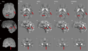

Figure 4 depicts two typical slices of reconstructed susceptibility maps by MEDI, EP-DL, and COSMOS methods, the top row [Figure 4A-4D] is the 80th slice, and the bottom row [Figure 4E-4H] the is 85th slice. With the COSMOS method used as the reference, we can observe in Figure 4 that the EP-DL method preserves structural details of the cortical ribbon while the MEDI method loses some tissue information (see the red arrows).
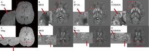
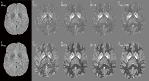
Figure 5 shows the reconstruction results of TKD method still have high noise, while the reconstruction results of MEDI and EP-DL method both have high reconstruction quality visually, and almost no artifacts can be observed for two data sets in the 2019 QSM reconstruction challenge.
Quantitative analysis
RMSE and HFEN with respect to the COSMOS method are calculated for quantitative performance evaluation (31). Here the RMSE is defined by Eq. [8]:
where χ is the recovered quantitative susceptibility map, with χR and ||·||F denoting the reference and the Frobenius-norm.
HFEN is defined by Eq. [9]:
where LoG is the Laplacian of the Gaussian operator.
The RMSE and HFEN values of the reconstructed susceptibility maps are summarized in Tables 2,3 for the TKD, MEDI and EP-DL methods.
Table 2
| Method | TKD | MEDI | EP-DL |
|---|---|---|---|
| RMSE | 69.9 | 74.5 | 56.8 |
| HFEN | 66.7 | 64.9 | 56.1 |
QSM, quantitative magnetic susceptibility mapping; EP-DL, edge prior guided dictionary learning; TKD, Thresholded K-space Division; MEDI, Morphology Enabled Dipole Inversion.
Table 3
| Method | TKD | MEDI | EP-DL | |
|---|---|---|---|---|
| 1 | RMSE | 75.0 | 40.5 | 39.5 |
| HFEN | 61.6 | 33.4 | 34.3 | |
| 2 | RMSE | 64.6 | 37.1 | 34.3 |
| HFEN | 63.2 | 30.6 | 30.5 | |
QSM, quantitative magnetic susceptibility mapping; EP-DL, edge prior guided dictionary learning; TKD, Thresholded K-space Division; MEDI, Morphology Enabled Dipole Inversion.
The results in Table 2 show that in the 2016 QSM reconstruction challenge data, the RMSE and HFEN of the EP-DL method are lower than the MEDI method, and the absolute improvements are 15.6% and 8.34% in terms of RMSE and HFEN, respectively.
Similarly, the EP-DL method also showed an advantage in the 2019 QSM reconstruction challenge data. For the first set, the quantitative indicators of EP-DL and MEDI were basically the same, and both were much lower than TKD. For the second set, the RMSE and HFEN of EP-DL were lower than those of TKD and MEDI.
In addition, Table 4 quantitatively evaluates the reconstruction performances of two slices showed in Figure 4. In the EP-DL method, the values of RMSE and HFEN are lower than the MEDI method. We also analyze the absolute values of the error in regions of interest (ROIs) for brain tissues of gray matter [globus pallidus (GP), putamen (PU), caudate nucleus (CN), red nucleus (RN), and substantia nigra (SN)] relative to the reference COSMOS data.
Table 4
| Method | MEDI | EP-DL | |||
|---|---|---|---|---|---|
| RMSE | HFEN | RMSE | HFEN | ||
| 80th slice | 69.4 | 62.7 | 56.4 | 55.4 | |
| 85th slice | 69.7 | 62.5 | 57.2 | 53.1 | |
QSM, quantitative magnetic susceptibility mapping; EP-DL, edge prior guided dictionary learning; MEDI, Morphology Enabled Dipole Inversion.
ROI_error is defined as:
where χROI is the ROI of recovered susceptibility map, χR_ROI is the ROI of reference and ROI_px is the pixel number of ROI. The range of the sum operation is the entire ROI.
Figure 6 depicts five selected ROI (Red is GP, blue is PU, green is CN, yellow is RN and pink is SN) of reconstructed susceptibility maps by MEDI, EP-DL, and COSMOS method. Table 5 lists the absolute value of the error of these ROIs, and we can observe that in the EP-DL method, the ROI error of GP, PU, CN, and RN are lower than the MEDI method.
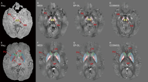
Table 5
| ROI | GP | PU | CN | RN | SN |
|---|---|---|---|---|---|
| MEDI | 0.030 | 0.019 | 0.016 | 0.022 | 0.056 |
| EP-DL | 0.029 | 0.011 | 0.008 | 0.014 | 0.068 |
QSM, quantitative magnetic susceptibility mapping; EP-DL, edge prior guided dictionary learning; MEDI, Morphology Enabled Dipole Inversion; GP, globus pallidus; PU. putamen; CN, caudate nucleus; RN, red nucleus; SN, substantia nigra.
Clinical GRE data results
Additionally, two sets of single orientation in vivo brain data are used in algorithm evaluation. 3T GRE data is obtained from Philips MRI platform with acquisition parameters: FOV: 230 mm × 230 mm × 126 mm, matrix size: 352×352×126, TR/TE1/∆TE: 50 ms/7.5 ms/7.2 ms, FA: 17° and echo number: 6. And 1.5 T GRE data is obtained from the XGY (an MRI equipment manufacturer in Ningbo, Zhejiang Province, China) MRI platform with acquisition parameters: FOV: 240 mm × 192 mm × 128 mm, matrix size: 256×205×64, TR/TE1/∆TE: 62 ms/7.1 ms/7.1 ms, FA: 15° and echo number: 4.
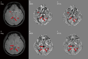
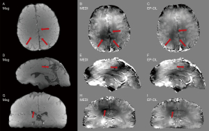
The EP-DL and the MEDI methods are used to reconstruct the susceptibility maps of these two datasets. In the experiments, we find that in the EP-DL method, setting λ2/λ1, block size and dictionary atom number are the same as in Table 1, and in the MEDI method, setting λ2 to 1,000 can get good results visually. Improved performance in artifact suppression is also validated by the visual results in Figure 7 (3T Philips clinical data) and Figure 8 (1.5T XGY clinical data) for the EP-DL method, and the susceptibility mapping results use the same parameters given in Section III. A. This also confirms the robustness when the same parameter setting is used for the same data type in the proposed algorithm.
Discussion
In the proposed method, the parameters (regularization parameters λ1 and λ2, block size N and dictionary atom number M2) are closely related to QSM reconstruction quality. Here the above parameters are analyzed with the other parameters fixed to the values given in Table 1. Experiment setting. Experiment results also confirm that the same parameter setting can be used for the same type of dataset.
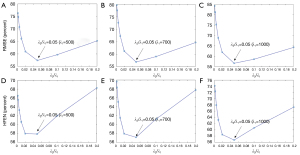
Eq. [5] has two regularization parameters λ1 and λ2, and the ratio between λ1 and λ2 needs to be well set to achieve a balance between different terms. With λ1 ranging from 500 to 1,000, Figure 9 shows that the lowest RMSE and HFEN can be obtained when λ2/λ1 equals to 0.05.
It can be observed in Figure 10 that the minimal RMSE and HFEN in the EP-DL method are obtained when λ1 is set to 1,100 and 1,300, respectively. And the minimal RMSE and HFEN in the MEDI method are obtained when λ1 equals 250 and 350, respectively.
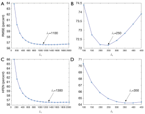
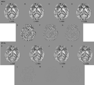
Nevertheless, in the experiment of 3T Philips data, when is set to 250, the MEDI method suffers from obvious over-smoothing (see in Figure 11). When varies from 600 to 1,400, the obvious difference can be observed between these reconstructed susceptibility maps (see in Figure 11). Here, we denote as the difference map, and are reconstructed results with regularization parameters and, respectively. In the EP-DL method (is fixed to 0.05), when the value of is set from 800 to 2,000, the variations of quantitative metrics are found to be small for the 2016 QSM challenge data. And the lowest RMSE and HFEN are obtained when equals 1,100 and 1,300 (see in Figure 10A,10C), respectively. In the experiment of 3T Philips data, in Figure 11, we can observe that in the EP-DL method, the reconstructed results are almost the same, and the difference between these susceptibility maps is smaller than the MEDI method.
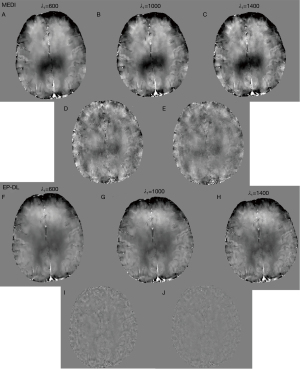
Moreover, in the experiment of 1.5T XGY data, in Figure 12, we can observe that when varies from 600 to 1,400, the difference between these reconstructed susceptibility maps by the MEDI method are obvious large than the EP-DL method (see the difference maps in Figure 12D,12E,12I,12J). Compared with the MEDI method, the proposed EP-DL method is found to be less sensitive to the regularization parameter when the parameter ratio is fixed.
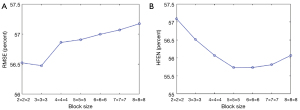
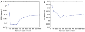
The analysis of the block size N and dictionary atom number is provided in Figure 13 and Figure 14. Figure 13 shows that the minimal RMSE and HFEN can be obtained when the block size is set to 3×3×3 and 5×5×5, respectively. And we observe that the distance between the highest and lowest value of RMSE and HFEN are 0.69 and 1.39, respectively. In Figure 14, we can see that the minimum RMSE and HFEN are reached when the dictionary atom number N is set to 300. We also find that the difference between the highest and lowest value of RMSE and HFEN are 0.23 and 0.19, respectively. Such results show that the parameters N and have little effect upon the reconstruction quality in terms of metrics RMSE and HFEN.
For the 2016 QSM challenge data, EP-DL took about 10 min to train the dictionary using an Intel(R) Core(TM) i7-6820HK CPU. In terms of reconstruction times, EP-DL took about 10 minutes to reconstruct the QSM image, and the method of MEDI reconstructing time was about 5 min.
Conclusions
In this paper, we propose an EP-DL method for dipole inversion in quantitative susceptibility mapping reconstruction. Improved performance in streaking artifacts suppression, structural recovery, deep gray matter reconstruction is obtained.
Future work will be focused on the evaluation of the effectiveness of the EP-DL method in patients with brain injuries such as micro-bleed multiple sclerosis lesions, hemorrhage, etc. To achieve a more robust QSM reconstruction, the adaptive parameters selection method needs to be developed for the data with different properties. Also, to meet the requirement of feasible applications, the iteration process needs to be accelerated by using parallelized computing architectures such as the Graphical Processing Unit (GPU).
Acknowledgments
Funding: This work was supported in part by the State's Key Project of Research and Development Plan under Grant 2017YFA0104302 and Grant 2017YFC0109202, in part by the National Natural Science Foundation under 61871117, in part by Science and Technology Program of Guangdong (2018B030333001).
Footnote
Conflicts of Interest: All authors have completed the ICMJE uniform disclosure form (available at https://dx.doi.org/10.21037/qims-21-243). The authors have no conflicts of interest to declare.
Ethical Statement: The authors are accountable for all aspects of the work in ensuring that questions related to the accuracy or integrity of any part of the work are appropriately investigated and resolved. The study was conducted in accordance with the Declaration of Helsinki (as revised in 2013). This study protocol was approved by the ethics committee of Southeast University, and written informed consent was obtained from each participant. All ethical guidelines were followed in our description of the experiments performed with human samples.
Open Access Statement: This is an Open Access article distributed in accordance with the Creative Commons Attribution-NonCommercial-NoDerivs 4.0 International License (CC BY-NC-ND 4.0), which permits the non-commercial replication and distribution of the article with the strict proviso that no changes or edits are made and the original work is properly cited (including links to both the formal publication through the relevant DOI and the license). See: https://creativecommons.org/licenses/by-nc-nd/4.0/.
References
- Haacke EM, Tang J, Neelavalli J, Cheng YC. Susceptibility mapping as a means to visualize veins and quantify oxygen saturation. J Magn Reson Imaging 2010;32:663-76. [Crossref] [PubMed]
- Wisnieff C, Ramanan S, Olesik J, Gauthier S, Wang Y, Pitt D. Quantitative susceptibility mapping (QSM) of white matter multiple sclerosis lesions: Interpreting positive susceptibility and the presence of iron. Magn Reson Med 2015;74:564-70. [Crossref] [PubMed]
- Wang Y, Liu T. Quantitative susceptibility mapping (QSM): Decoding MRI data for a tissue magnetic biomarker. Magn Reson Med 2015;73:82-101. [Crossref] [PubMed]
- Dimov AV, Liu Z, Spincemaille P, Prince MR, Du J, Wang Y. Bone quantitative susceptibility mapping using a chemical species-specific R2* signal model with ultrashort and conventional echo data. Magn Reson Med 2018;79:121-8. [Crossref] [PubMed]
- Wong R, Chen X, Wang Y, Hu X, Jin MM. Visualizing and quantifying acute inflammation using ICAM-1 specific nanoparticles and MRI quantitative susceptibility mapping. Ann Biomed Eng 2012;40:1328-38. [Crossref] [PubMed]
- Azuma M, Hirai T, Yamada K, Yamashita S, Ando Y, Tateishi M, Iryo Y, Yoneda T, Kitajima M, Wang Y, Yamashita Y. Lateral Asymmetry and Spatial Difference of Iron Deposition in the Substantia Nigra of Patients with Parkinson Disease Measured with Quantitative Susceptibility Mapping. AJNR Am J Neuroradiol 2016;37:782-8. [Crossref] [PubMed]
- Liu T, Surapaneni K, Lou M, Cheng L, Spincemaille P, Wang Y. Cerebral microbleeds: burden assessment by using quantitative susceptibility mapping. Radiology 2012;262:269-78. [Crossref] [PubMed]
- Sharma SD, Hernando D, Horng DE, Reeder SB. Quantitative susceptibility mapping in the abdomen as an imaging biomarker of hepatic iron overload. Magn Reson Med 2015;74:673-83. [Crossref] [PubMed]
- Sun H, Klahr AC, Kate M, Gioia LC, Emery DJ, Butcher KS, Wilman AH. Quantitative Susceptibility Mapping for Following Intracranial Hemorrhage. Radiology 2018;288:830-9. [Crossref] [PubMed]
- de Rochefort L, Liu T, Kressler B, Liu J, Spincemaille P, Lebon V, Wu J, Wang Y. Quantitative susceptibility map reconstruction from MR phase data using bayesian regularization: validation and application to brain imaging. Magn Reson Med 2010;63:194-206. [Crossref] [PubMed]
- Wharton S, Schäfer A, Bowtell R. Susceptibility mapping in the human brain using threshold-based k-space division. Magn Reson Med 2010;63:1292-304. [Crossref] [PubMed]
- Li W, Wang N, Yu F, Han H, Cao W, Romero R, Tantiwongkosi B, Duong TQ, Liu C. A method for estimating and removing streaking artifacts in quantitative susceptibility mapping. Neuroimage 2015;108:111-22. [Crossref] [PubMed]
- Schweser F, Sommer K, Deistung A, Reichenbach JR. Quantitative susceptibility mapping for investigating subtle susceptibility variations in the human brain. Neuroimage 2012;62:2083-100. [Crossref] [PubMed]
- Fong D, Saunders M. LSMR: an iterative algorithm for sparse least-squares problems. SIAM J Sci Comput 2011;33:2950-71. [Crossref]
- Langkammer C, Bredies K, Poser BA, Barth M, Reishofer G, Fan AP, Bilgic B, Fazekas F, Mainero C, Ropele S. Fast quantitative susceptibility mapping using 3D EPI and total generalized variation. Neuroimage 2015;111:622-30. [Crossref] [PubMed]
- Wei H, Dibb R, Zhou Y, Sun Y, Xu J, Wang N, Liu C. Streaking artifact reduction for quantitative susceptibility mapping of sources with large dynamic range. NMR Biomed 2015;28:1294-303. [Crossref] [PubMed]
- Liu Z, Kee Y, Zhou D, Wang Y, Spincemaille P. Preconditioned total field inversion (TFI) method for quantitative susceptibility mapping. Magn Reson Med 2017;78:303-15. [Crossref] [PubMed]
- Sun H, Ma Y, MacDonald ME, Pike GB. Whole head quantitative susceptibility mapping using a least-norm direct dipole inversion method. Neuroimage 2018;179:166-75. [Crossref] [PubMed]
- Liu T, Liu J, de Rochefort L, Spincemaille P, Khalidov I, Ledoux JR, Wang Y. Morphology enabled dipole inversion (MEDI) from a single-angle acquisition: comparison with COSMOS in human brain imaging. Magn Reson Med 2011;66:777-83. [Crossref] [PubMed]
- Liu T, Wisnieff C, Lou M, Chen W, Spincemaille P, Wang Y. Nonlinear formulation of the magnetic field to source relationship for robust quantitative susceptibility mapping. Magn Reson Med 2013;69:467-76. [Crossref] [PubMed]
- Liu T, Spincemaille P, de Rochefort L, Kressler B, Wang Y. Calculation of susceptibility through multiple orientation sampling (COSMOS): a method for conditioning the inverse problem from measured magnetic field map to susceptibility source image in MRI. Magn Reson Med 2009;61:196-204. [Crossref] [PubMed]
- Yoon J, Gong E, Chatnuntawech I, Bilgic B, Lee J, Jung W, Ko J, Jung H, Setsompop K, Zaharchuk G, Kim EY, Pauly J, Lee J. Quantitative susceptibility mapping using deep neural network: QSMnet. Neuroimage 2018;179:199-206. [Crossref] [PubMed]
- Bollmann S, Rasmussen KGB, Kristensen M, Blendal RG, Østergaard LR, Plocharski M, O'Brien K, Langkammer C, Janke A, Barth M. DeepQSM - using deep learning to solve the dipole inversion for quantitative susceptibility mapping. Neuroimage 2019;195:373-83. [Crossref] [PubMed]
- Liu J, Chen Y, Hu Y, Luo L. Low-dose CBCT reconstruction via 3D dictionary learning. 2016 IEEE 13th International Symposium on Biomedical Imaging (ISBI), Prague, pp. 735-738, Apr. 2016.
- Chen Y, Shi L, Feng Q, Yang J, Shu H, Luo L, Coatrieux JL, Chen W. Artifact suppressed dictionary learning for low-dose CT image processing. IEEE Trans Med Imaging 2014;33:2271-92. [Crossref] [PubMed]
- Liu J, Hu Y, Yang J, Chen Y, Shu H, Luo L, Feng Q, Gui Z, Coatrieux G. 3D Feature Constrained Reconstruction for Low Dose CT Imaging. IEEE Transactions on Circuits and Systems for Video Technology 2018;28:1232-47. [Crossref]
- Liu J, Ma J, Zhang Y, Chen Y, Yang J, Shu H, Luo L, Coatrieux G, Yang W, Feng Q, Chen W. Discriminative Feature Representation to Improve Projection Data Inconsistency for Low Dose CT Imaging. IEEE Trans Med Imaging 2017;36:2499-509. [Crossref] [PubMed]
- Ravishankar S, Bresler Y. MR image reconstruction from highly undersampled k-space data by dictionary learning. IEEE Trans Med Imaging 2011;30:1028-41. [Crossref] [PubMed]
- Zhuang P, Zhu X, Ding X. MRI reconstruction with an edge-preserving filtering prior. Signal Processing 2019;155:346-57. [Crossref]
- Iyer SK, Tasdizen T, Dibella E. Edge-enhanced spatiotemporal constrained reconstruction of undersampled dynamic contrast-enhanced radial MRI. Magn Reson Imaging 2012;30:610-9. [Crossref] [PubMed]
- Langkammer C, Schweser F, Shmueli K, Kames C, Li X, Guo L, Milovic C, Kim J, Wei H, Bredies K, Buch S, Guo Y, Liu Z, Meineke J, Rauscher A, Marques JP, Bilgic B. Quantitative susceptibility mapping: Report from the 2016 reconstruction challenge. Magn Reson Med 2018;79:1661-73. [Crossref] [PubMed]
- Elad M, Aharon M. Image denoising via sparse and redundant representations over learned dictionaries. IEEE Trans Image Process 2006;15:3736-45. [Crossref] [PubMed]
- Rubinstein R, Zibulevsky M, Elad M. Efficient implementation of the K-SVD algorithm using batch orthogonal matching pursuit. CS Technion 2008;40:1-15.
- Jenkinson M, Beckmann CF, Behrens TE, Woolrich MW, Smith SM. FSL. Neuroimage 2012;62:782-90. [Crossref] [PubMed]
- Schofield MA, Zhu Y. Fast phase unwrapping algorithm for interferometric applications. Opt Lett 2003;28:1194-6. [Crossref] [PubMed]
- Zhou D, Liu T, Spincemaille P, Wang Y. Background field removal by solving the Laplacian boundary value problem. NMR Biomed 2014;27:312-9. [Crossref] [PubMed]


