
State-of-the-art in retinal optical coherence tomography image analysis
Introduction
Optical coherence tomography (OCT) is a powerful imaging system for acquiring 3D volumetric images of tissues non-invasively. In simple terms, OCT can be considered as echography with light (1). Unlike echography which is done by sound waves, OCT imaging is not time-of-flight based but rather produces the image based on the interference patterns. Figure 1 shows a typical retinal OCT image with false color. Throughout the past two decades, new developments in the OCT imaging system have improved the acquisition time and also the quality of the acquired images. Nowadays taking µm-level volume images of the tissues is very common especially in ophthalmology and retinal imaging. Due to the volume of data generated in a clinical setting, there is a need for robust and automated analysis techniques to fully leverage the capabilities of OCT imaging (3).

In this paper we will discuss the three main aspects of automated retinal OCT image processing: noise reduction, segmentation and image registration. The process of OCT image acquisition results in the formation of irregular granular pattern called speckle. Speckle degrades the quality of the image and affects subsequent processing and analysis. Therefore, the first step in OCT image processing involves attenuation of speckle.
Delineating micro-structures in the image is of particular importance in OCT image processing for ophthalmology. For example, measuring the thickness of various layers in the retina is important for early diagnosis and tracking of diseases such as glaucoma. Therefore image segmentation plays a significant role in OCT image analysis. Moreover, given that OCT imaging is used to study microscopic feature sizes, minor fixation instability during image acquisition can grossly affect image quality. With hundreds of cross-sectional slices being acquired to construct volumetric data, eye movements can affect alignment of these slice images. Furthermore, image registration may also be used in tracking the progress of tissue degeneration over time.
This article is organized as follows: section 2 is an overview of OCT imaging and different techniques that are used to acquire and reconstruct the images. Section 3 focuses on noise reduction techniques. In section 4, a few techniques for OCT image segmentation, with a focus on retinal layer segmentation are reviewed. Section 5 contains an overview of the use of image registration techniques in OCT image analysis. Finally, section 6 concludes the article with pointers on some of the future paths that can be taken for further investigations.
OCT imaging systems
OCT imaging is based on the interference pattern between a split and later re-combined broadband optical field (3). Figure 2 displays a typical OCT imaging system. The light beam from the source is exposed to a beam splitter and travels in two paths: one toward a moving reference mirror and the other to the sample to be imaged. The reflected light from both the reference mirror and the sample are fed to a photo detector in order to observe the interference pattern. The sample usually contains particles (or layers) with different refractive indices and the variation between their differences causes intensity peaks in the interference pattern detected by the photo detector.

The first widely available OCT imaging system in biomedical imaging is called time-domain OCT (TD-OCT) in which a reference mirror is translated to match the optical path from reflections within the sample (2). TD-OCTs usually use a super luminescent diode (SLD) as the light source (3). Unlike the TD-OCT, in Fourier-domain OCT (FD-OCT) there is no need for moving parts in the design of the imaging system to obtain the axial scans (4) since the reference path length is fixed and the detection system is replaced with a spectrometer. Considering a 50:50 beam-splitter and after some simplifications, the expression for the detected frequency spectrum can be expressed as (3):

where  is the intensity spectrum and
  is the sample’s frequency domain response function. The time domain interference pattern can be derived using an N point discrete fast Fourier transform (FFT), each point being corresponding to an intensity measurement at each detector in the detector array. The rate at which the data can be transferred from the detector to the computer can have a big impact on the scan rate. With one dimensional detectors, this is not usually the problem, but using 2D detectors requires massive transfer rates, in the order of several gigabytes per second. The use of CCD sensors for buffering the data during the scan and retrieving it at a later time can be useful as been previously mentioned in (3). Of course other configurations of FD-OCT can be used. Swept-Source OCT (SS-OCT) is one of the very well-known and widely used FD-OCTs in which using a single detector allows for the source spectrum to be swept and the intensity of component frequency to be detected (5). Overall, because of not having any moving parts, the speed of FD-OCT systems in acquiring images is very high in comparison to TD-OCT.
Quantum OCT (Q-OCT) takes advantage of quantum nature of light, rather than its classical behavior, for imaging (6). Full field OCT (FF-OCT) is another optical coherence imaging technique in which a CCD camera is placed at the output, instead of the single detector of the TD-OCT, to capture a 2D en face image in a single exposure (7). Taking into account the polarization state of the light, polarization-sensitive OCT (PS-OCT) is another technique for imaging the birefringence within a biological sample (8). Doppler OCT (D-OCT) which is also called optical Doppler tomography (ODT) is a combination of an OCT imaging system and laser Doppler flowmetry. This system allows for the quantitative imaging of fluid flow in a highly scattering medium; such as monitoring in vivo blood flow beneath the skin (9). Discussing these different OCT imaging systems is not the main focus of the current work and therefore, the reader is referred to (3,10-12).
Noise reduction
Speckle is a fundamental property of signals and images acquired by narrow-band detection systems like Synthetic Aperture Radar (SAR), ultrasound and OCT. In OCT, not only the optical properties of the system, but also the motion of the subject to be imaged, size and temporal coherence of the light source, multiple scattering, phase deviation of the beam and aperture of the detector can affect the speckle (13). Two main processes affect the spatial coherence of the returning light beam which is used for image reconstruction: (I) multiple back-scattering of the beam; and (II) random delays for the forward-propagating and returning beam caused by multiple forward scattering. In the case of tissue imaging, since the tissue is packed with sub-wavelength diameter particles which act as scatterers, both of these phenomena contribute to the creation of speckle. As been previously studied (13), two types of speckle are present in OCT images: signal-carrying speckle which originates from the sample volume in the focal zone; and signal-degrading speckle which is created by multiple-scattered out-of-focus light. The latter kind is what that is considered as speckle noise. Figure 3 displays the common scene in retinal OCT imaging; a highly noisy image.

The distribution of the speckle can be represented with a Rayleigh distribution. Speckle is considered as a multiplicative noise, in contrast to Gaussian additive noise. Due to the limited dynamic range of displays, OCT signals are usually compressed by a logarithmic operator applied to the intensity information. Following this, the multiplicative speckle noise is transformed to additive noise that can be further treated (14).
OCT noise reduction techniques can be divided into two major classes: (I) methods of noise reduction during the acquisition time and (II) post-processing techniques. In the first class, compounding techniques, multiple uncorrelated recordings are averaged. Among them, spatial compounding (15), angular compounding (16), polarization compounding (17) and frequency compounding (18) can be mentioned. Usually the methods from the first class are not preferred since they require multiple scanning of the same data which prolongs the acquisition time. In addition, these techniques can be very restrictive in terms of different OCT imaging systems in use. Therefore, use of more general post-processing techniques is more favorable. In the literature, many of post-processing methods have been proposed for speckle noise reduction of OCT images. There are few classic techniques for noise reduction that are successfully used in OCT images: Lee (19), Kuan et al. (20) and Frost et al. (21) filters.
The class of methods for speckle reduction based on the well-known anisotropic diffusion method (22) is of high interest in the literature. The nonlinear Partial Differential Equation (PDE) for smoothing the image I can be formulated as follows:

where  is the gradient operator, div is the divergence operator,
  represents the magnitude and d(x) is the diffusion coefficient. The initial condition for this PDE is
  Different types of functions considered for d(x) result in different types of filters. Choosing the diffusion coefficient function to be constant results in a linear diffusion equation with homogeneous diffusivity which its solution is equivalent to smoothing the image with a Gaussian filter. In this case, the filter makes the noise within regions smoother, while blurring the edges at the same time. Making the diffusion coefficient image dependent results in a nonlinear diffusion equation. Due to its poor performance in the case of very noisy images, there are different variations of this method in the literature (23-25). In (14) a complete comparison is provided for regular anisotropic diffusion and complex anisotropic diffusion approaches for denoising of OCT images. For the nonlinear complex diffusion, the equation is as follows:

where  is the imaginary value and the diffusion coefficient is defined as:
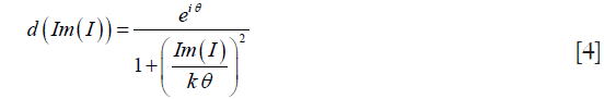
with k being the threshold parameter and  being the phase angle. A smooth second derivative of the image factored by θ at time t is considered as the imaginary part in the above equations. This serves as a robust edge detector which provides better performance in comparison to the regular nonlinear diffusion approach.
Another example of using anisotropic diffusion is in (26) where an interval type-II fuzzy approach is used for determining the diffusivity function of the anisotropic diffusion. Starting from a Prewitt operator for detecting the edges in the image followed by Gaussian and median filtering, the process of defining the diffusion coefficient is carried out by first determining two linguistic variables, edge value and noise level. This results in the definition of two fuzzy variables; edginess measure and noisiness measure. After assigning the membership functions to these variables, with added uncertainty of course, the fuzzy set of rules is defined. Here, only one rule suffices: IF edginess measure is low AND noisiness measure is high, THEN the diffusion coefficient has a high value. Finally the diffusion coefficient is derived by type reducing and de-fuzzifying of the output of the fuzzy system and is used for finding the solution of the anisotropic diffusion process.
Another important group of widely used methods for de-speckling of OCT images takes advantage of multiscale/multiresolution geometric representation techniques (1,27). The main reason for this is that these representations compress the essential information of the image into a few large coefficients while noise is spread among all of the coefficients. Generally, for such methods a transform domain that provides a sparse representation of images and an optimal threshold is needed. Using the optimal threshold, hard- or soft-thresholding can be done for coefficient shrinkage in order to reduce the noise. This threshold can be a constant or even better, sub-band adaptive or spatially adaptive. For example, in OCT images, since it is known that most of the features are horizontal, higher thresholds can be applied to the vertical coefficients. Wavelet transform is one example of such methods which has been widely used in this area (28). Applying this wavelet transform on the logarithmic image in which the multiplicative noise is transformed to an additive noise, the wavelet coefficients are extracted as:

where  are the noise-free coefficients,
  the noise contribution, o the sub-band orientation, j the decomposition level and k the spatial coordinate. Taking a soft-thresholding approach with
  as threshold, the new set of wavelet coefficients can be derived as:

The threshold is computed based on the ratio of the noise variance to the standard deviation of the Generalized Gaussian Distribution (GGD) random variables that describe the noise free coefficients. The final result is reconstructed by simply performing the inverse wavelet transform. Even though wavelet transform has shown promising results, its lack of directionality imposes some limitations in properly denoising OCT images. This can be further improved by use of dual-tree complex wavelet transform (DT-CWT) which doubles the directional information of wavelet transform (29). Still, there are better transform domains which offer more proper representations for OCT images. In the past few years, the use of Curvelet transform (30,31), Contourlet transform (32,33) and Ripplet transform (34) showed promising results in the de-noising of OCT images, with the procedure almost the same as the method mentioned above, with slight differences regarding the type of threshold (hard or soft) and the method of defining the threshold. Figure 4 shows the result of curvelet coefficients shrinkage for speckle noise reduction.

Compressive sensing and sparse representation are new directions that are taken for image acquisition and noise reduction. Very recent examples (35,36) use dictionary learning and sparse representation for noise reduction and image reconstruction of OCT. To be more detailed, sparse representation tries to approximate an image by a weighted average of a limited number of basic elements (atoms) from a learned dictionary of basis functions. Representing an image patch X of size n×m as a vector x of size q=n×m, the dictionary  containing k atoms is used to approximate the patch as
  , while
  , ε being the error tolerance and
  representing the p-norm. Choosing the proper dictionary results in having a sparse coefficient vector α which means that
  . The process of dictionary learning is a generalization from methods mentioned previously in which the set of atoms (wavelet, curvelet, contourlet, ripplet atoms) could be represented mathematically. Here, the procedure involves using a set of example patches and minimizing the following problem:

with Z being the number of patches and T being the sparsity level. The sparse representation-based method proposed in (36) starts with registering and averaging slices (considering one of them as target) of the same cross-section in the retina to create the desired high-SNR-high-resolution (HH) image and down-sampling the target slice to create the low-SNR-low-resolution (LL) image, SNR being Signal-to-Noise Ratio. Then for each one, the corresponding dictionary DH,H and DL,L is learned utilizing Coupled Orthogonal Matching Pursuit (COMP) method, a variation of Orthogonal Matching Pursuit (OMP) (37), a method widely used in the field of sparse representation. This is followed by finding the mapping between the coefficient vectors of the dictionaries by solving a ridge regression problem. In the image reconstruction phase, DL,L is used for extracting the coefficient vectors of the observed LL patches. The HH patch is reconstructed using DH,H and the mapping found in the previous step. To make the dictionary learning process more efficient, training patches from both LL and HH are clustered into several structural clusters, and for each a compact dictionary and mapping function is learned and then used. For 3D reconstruction, after registering the slices together to compensate for the effect of eye movements and assuming that similar patches from nearby slices can be represented by the same atoms from dictionaries, Simultaneous Orthogonal Matching Pursuit (SOMP) algorithm (38) is used for approximating the coefficient vectors for LL. The corresponding HH dictionary and the mapping function are then used for approximating the HH patches. These patches are then used for reconstruction of the final images.
Image segmentation
Image segmentation is a very active area in the field of medical image analysis. The most difficult step in any medical image analysis system is the automated localization and extraction of the structures of interest (39). The signal strength in OCT images rises from the intrinsic differences in optical properties of tissues. In the retina, multiple layers of different types of cells can be seen in OCT images. During the last two decades many methods have been proposed for segmentation of OCT images. For a more complete review on the methods the reader is referred to (39-41). There are four major hurdles that are encountered in the segmentation of OCT images:
- The presence of speckle noise complicates the process of the precise identification of the retinal layers, therefore most of the segmentation methods require pre-processing steps to reduce the noise;
- Intensity of homogeneous areas decreases with increased depth of imaging. This is due to the fact that the intensity pattern in OCT images is the result of the absorption and scattering of light in the tissue;
- Optical shadows imposed by blood vessels can also affect the performance of segmentation methods;
- Quality of OCT images degrades as a result of motion artifacts or sub-optimal imaging conditions.
Methods of retinal segmentation can be categorized into five classes: (I) methods applicable to A-scans; (II) intensity-based B-scans analysis; (III) active contour approaches; (IV) analysis methods using artificial intelligence and pattern recognition techniques; and (V) segmentation methods using 2D/3D graphs constructed from the 2D/3D OCT images (41,42).
A-scan based methods consider the difference in the intensity levels to extract the edge information. Due to the effects of speckle noise, these methods are usually used for determining the most significant edges on the retina. Examples of such methods are presented in (2,43-46). A-scan based methods lack the contribution from 2D/3D data while the computational time is high and the accuracy is low. Taking advantage of better de-noising methods, intensity-based B-scan analysis approaches are based on the intensity variations and gradients which are still too sensitive and make these methods case-dependent (47-49).
Active contour methods also provide promising results for segmentation of retinal layers in OCT images. Methods presented in (50), (51) and (52) are three well-known examples. General active contour method proposed by (53) consists of an energy minimizing spline v(s) for s∈[0,1] for the energy functional:
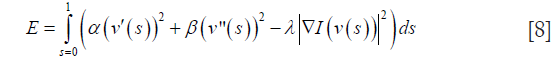
with α, β and λ being the weight constants and I being the gradient of the image. Here  represents the internal energy which imposes the piecewise smoothness constraint of the spline while
  , representing the external energy, and acts as a guidance for pushing the active contour (snake) toward salient image features like edges or lines etc.
In (52), the objective is segmenting the image domain (retinal B-scan) into disjoint sub-regions, representing retinal layers using a level-set framework as a set of R−1 signed distance functions (SDFs) named ø which determine the distance from any point in the image domain to the object boundary. The energy functional in its general form can be defined as:

EI being the image region-based information ensuring to have approximately constant intensity in each region, ES being the prior shape knowledge of retinal layer and ER being the regularization term for keeping the boundaries smooth.
Use of pattern recognition based methods is a new direction that attracted researchers for more explorations. In (54) a support vector machine (SVM) is used to perform the semi-automatic segmentation of retinal layers. For SVM, the radial basis kernel is used. As for the vector space for classification, a combination of the voxel’s intensity value, spatial location of the voxel, mean and variance of a small region surrounding the voxel in question and the gradient based on a local difference operator is considered. To make the algorithm more robust to different distributions of data intensities, a multi-resolution hierarchical representation of the OCT data is used and the final input vector is computed as a weighted average of the feature vectors at each level of the hierarchy. The next steps are providing the training data by the user for training the SVM classifier followed by segmentation of the retinal layers. In (55) fuzzy C-means clustering method is used for layer segmentation. The use of random forest classifier for segmentation is also reported in (56). In this study at first the intensities are normalized and then using an A-scan based technique, inner limiting membrane (ILM) and Bruch’s membrane (BrM) layers are extracted to be used for flattening the images with respect to the BrM layer. The next step is computing a set of 27 features to be fed into the Random Forest (RF) classifier which has been already trained using the labeled ground truth data provided by the user. The output of the classifier will be the boundary probabilities at every pixel. Finally, the segmentation results will be generated from the boundary probabilities and some boundary refinement algorithm.
Tow/three dimensional (2D/3D) graph-based methods are probably the best among all of the segmentation methods since they are relatively fast, more accurate and unlike the classification based techniques, don’t need training datasets for segmentation of new datasets. During the past few years several variations of this class were introduced in the literature. Examples of such methods can be found in (42,57-60). The method in (42) is based on diffusion maps (61) and takes advantage of regional image texture rather than edge information. Therefore it is more robust in low contrast and poor layer-to-layer image gradients. Diffusion maps can be considered as a method for dimentionality reduction and manifold learning which tries to extract the underlying manifold in the dataset to be used in reducing the dimentionality. In (42) two cascaded diffusion maps are used for segmentation of retinal layers. Starting from a square grid on the image data and considering the location of the centroid of each block and the mean value of the pixels contained in it as features, the graph is built and diffusion coordinates are extracted. Applying the K-means clustering on the results of the previous step will provide us with the approximate locations of 1st and 7th boundaries. After moving these points to their correct locations using a gradient-based technique and smoothing, 8th-11th boundaries are located by searching for locations with highest/lowest gradient values below the 7th boundary. After alignment with respect to the 10th boundary and limiting the search region to the region between 1st and 7th boundaries, thin non-overlapping rectangular blocks are chosen to be used for the next diffusion map and diffusion coordinate extraction which results in detecting 2nd-6th boundaries.
On the other hand, methods presented in (58-60) use the graph-cuts and shortest path method for segmentation of retinal layers. Considering image pixels as nodes of a graph, the weights between the nodes are assigned based on a priori information about the layer boundaries. The weight between nodes a and b is defined as:

where gi is the normalized vertical gradient of the image at node  ,
,  is the similarity factor weight, ij is the normalized intensity of node ,
  is the vertical penalty term and finally
  is the minimum weight added for numerical stability. After denoising the OCT volume using 3D block matching filter (BM3D) and the sparse representation-based technique introduced in (36), SVM classification is used to distinguish between volumes containing either 8 or 10 layers of the retina which is followed by the routines for segmenting retinal layers, optic nerve head and blood vessels’ segmentation. Figure 5 shows a few examples of the results of the method in (60).

Despite the plethora of different methods in this area, retinal layer segmentation is still an open problem with lots of room for improvement, especially in case of pathological eyes which introduce more challenges for segmentation.
Image registration
Having two input images, a template image and a reference image, image registration tries to find a valid optimal spatial transformation to be applied to the template image to make it more similar to the reference image (62,63). Therefore, the process of image registration consists of an optimization process fulfilling some imposed constraints. The applications of medical image registration range from mosaicing of retinal images (64) to slice interpolation (65).
There are two different classes of image registration techniques: (I) parametric approaches and (II) non-parametric approaches (66). In general, the process of finding the valid optimal spatial transformation can be formulated as
There are several different applications for using image registration approaches in OCT image analysis. One of the basic applications is in speckle noise reduction. As mentioned in Section 3, hardware-based noise reduction techniques take the average of several uncorrelated scans in order to reduce the noise. The same thing can happen after finishing image acquisition too. The main idea is to gather several images of the same cross-section of the retina, register them together and take the average/median. A slight movement of the eye provides us with an uncorrelated pattern of speckle. Having N B-scans, the SNR can be improved by a factor of sqrt(N). In (68) a dynamic programming-based method is used for compensation of the movements between several B-scans and reducing the speckle noise. A hierarchical model-based motion estimation scheme based on an affine-motion model is used in (69) for registering multiple B-scans to be used for speckle reduction. In (70) a rigid registration technique is used for alignment of the B-scans and the final denoised image is obtained using various Independent Component Analysis (ICA) techniques for comparison. Recently, the use of low-rank/sparse decomposition based batch alignment has been investigated for speckle noise reduction in OCT images too. Taking advantage of Robust Principal Component Analysis (RPCA) (71) and simultaneous decomposition and alignment of a stack of OCT images via linearized convex optimization, better performance is achieved in comparison to previous registration-based de-noising techniques (72,73). Assuming N B-scans from the same location in the retina (to some extent), data matrix D is created by stacking the vectorized images as columns of the matrix. Having perfectly aligned B-scans results in D being decomposable into two components: D=L+S, L being low-rank containing the desired noise-free image and S being sparse containing only speckle noise. But due to eye movements, a set of parametric transformations τ are also needed to be considered, which makes the optimization problem for simultaneous alignment and decomposition as follows:

where  is the nuclear norm (sum of singular values) and
  is the l1 norm. Linearizing the constraint with the assumption of having minimal changes in τ at each iteration and using Augmented Lagrange Multiplier (ALM) (74) are next steps for simultaneous alignment and low-rank/sparse decomposition of the set of B-scans. Figure 6 shows the result of the method using 50 misaligned macular B-scans.

Another application is in the registration of fundus images with en face OCT images. This is very helpful to better correlate retinal features across different imaging modalities. In (75) an algorithm is proposed for registering OCT fundus images with color fundus photographs. In that study, blood vessel ridges are taken as features for registration. A similar approach is taken in (76) too. Using the curvelet transform, the blood vessels are extracted for the two modalities. The process of blood vessel extraction involves curvelet-based contrast enhancement, match filtering for intensifying the blood vessels, curvelet-based vessel segmentation followed by length filtering for removing the misclassified pixels. The image registration procedure is done in two steps. In the first step, an approximate for the central part of both the en face OCT and color fundus is estimated. This is followed by defining a search area in the fundus image and trying to find the best match of the two vessel images using the similarity measure as follows:

where A and B are the vessel patterns of the en face OCT and fundus images, respectively. The next step is using a quadratic transformation model for registering the two vessel images since the retina is assumed to be a second-order surface. Figure 7 shows different stages of the results of color fundus and en face OCT image registration of the method proposed in (75).

Motion correction of OCT images is another area in which image registration techniques are of high interest. There are several different involuntary eye movements that can happen during the fixation: tremor, drifts and micro-saccades (77). One way to deal with this issue is a hardware solution which involves having eye tracking equipment to compensate for eye movements during image acquisition. Usually a Scanning Laser Ophthalmoscopy (SLO) device is merged with the OCT for tracking these eye movements during imaging (78). Taking a software approach can be more general and applicable without the need for additional imaging equipment. In (79) at first the vessels are detected in both SLO and en face OCT, using hysteresis thresholding for finding ridges in the normalized divergence of the image gradient followed by eliminating regions of less than five pixels. For correcting the tremors and drifts an elastic image registration with local affine model is considered (80). Micro-saccades are corrected in the next step by finding the horizontal shift at each pixel in the scan that best aligns the result of tremor and drift corrected image with the SLO image. In (81) a 3D aligning method for motion correction is proposed based on particle filtering. Particle filtering is an effective approach for target tracking which is based on the idea of considering the target as a state space model and converting the tracking to a state estimation problem. In this work, two consecutive motion correction based on particle filtering are implemented for 3D motion correction. In (82), 2 volume scans with orthogonal fast scan axes are used for motion correction in 3D on a per A-scan basis. The proposed technique is implemented in a multi-resolution based manner to ensure less computational time. In order to account for the variations in illumination and also the effect of speckle noise in the process, in (83) a more robust similarity measure for optimization is proposed based on a modified version of Pseudo-Huber loss function (84) which is less sensitive to outliers than squared error loss. Figure 8 shows one example of using the algorithm in (82) to correct for the motion in OCT images.

Image mosaicing is another example of using image registration methods in OCT image processing. OCT systems are capable of acquiring a huge amount of data in a very short period of time; but still, the field of view is very limited. Stitching several volume data from a patient can improve the interpretation of data significantly. Usually in such methods, a set of overlapping OCT data is acquired and then stitched together using global/local image registration techniques. In (85) a set of 8 overlapping 3D OCT volume data is acquired over a wide area of retina. Then the OCT en face fundus images are registered together using blood vessel ridges as distinctive features of interest. As for a pre-processing step, Retinal Pigment Epithelium (RPE) layer is segmented as the second peak in each A-scan when starting from the top. This will help in creating a better en face OCT image with higher contrast for distinguishing the blood vessels. Finally the 3D OCT data sets are merged together using a combination of resampling, interpolation and cross-correlation. A relatively similar approach is taken in (86) too for motion correction and 3D volume mosaicing of OCT images. The whole procedure involves motion detection and image sub-division in a strip-based manner followed by Gabor filtering, zero-padding and initial strip placement. For global registration of the strips, a FFT-based correlation maximization algorithm (87) is used which is followed by a local B-spline registration technique for better alignment of the image features (blood vessels). Finally the composite image is created combining the results of global and local registrations. Figure 9 shows a color encoded depth image of the retina with three main vessel layers created using this method. One of the very recent works in this area can be found in (88) for bladder OCT images which is used with an integrated White Light Cystoscopy (WLC) system.

The use of image registration techniques in analysis and processing of OCT images has grown significantly in the past few years. Here only a few areas were mentioned and there are more to explore.
Conclusions
Even though the techniques introduced here do not represent a comprehensive list of all of the approaches that are used for analysis of OCT images, the variety of the techniques gives us some pointers on the possible directions for further explorations. With the emergence of parallel computing and GPU programming in the past few years, it is possible to have real time pre-processing and analysis systems to help with the increasing amount of data produced by OCT imaging systems. As for the pre-processing step, more robust and real-time techniques for speckle noise reduction and artifact (e.g., light strikes and blood vessel shadows) removal are needed. For segmentation, pixel/region classification-based techniques show promising results and are less affected by the noise and artifacts. The same goes for the introduction of more robust and accurate image registration techniques in analysis and interpretation of OCT data, for better understanding the process of tissue degeneration, inter-modality registration and real-time motion correction.
In this article, an overview of three major problems in OCT image analysis, namely noise reduction, image segmentation and image registration, is provided and several different techniques in each category are discussed. Starting from noise reduction, both hardware and software techniques are discussed to some extent. Moving to image segmentation, different segmentation techniques with a focus on retinal layer segmentation are introduced. Finally some of the image registration methods that are used for noise reduction, motion correction and image mosaicing of OCT images are reviewed. Overall, the use of image analysis techniques for OCT is a rapidly growing field and there remain many areas for investigation. The reader is referred to (89-95) for newer research that has been done in this area.
Acknowledgements
The authors would like to thank Dr. Joseph Carroll, Dr. Moataz M. Razeen and Dr. Yusufu Sulai from Advanced Ocular Imaging Program (AOIP: http://www.mcw.edu/AOIP.htm) for their valuable comments for improving the work.
Funding: This work was partially supported by NIH P30EY001931. Support received by grant 8UL1TR000055 from the Clinical and Translational Science Award (CTSA) program of the National Center for Research Resources and the National Center for Advancing Translational Sciences. Support received by the Clinical & Translational Science Institute of Southeast Wisconsin through the Advancing a Healthier Wisconsin endowment of the Medical College of Wisconsin.
Footnote
Conflicts of Interest: The authors have no conflicts of interest to declare.
References
- Pizurica A, Jovanov L, Huysmans B, Zlokolica V, De Keyser P, Dhaenens F. Multiresolution Denoising for Optical Coherence Tomography: A Review and Evaluation. Current Medical Imaging Reviews 2008;4:270-84.
- Huang D, Swanson EA, Lin CP, Schuman JS, Stinson WG, Chang W, Hee MR, Flotte T, Gregory K, Puliafito CA, et al. Optical coherence tomography. Science 1991;254:1178-81. [PubMed]
- Tomlins PH, Wang RK. Theory, developments and applications of optical coherence tomography. J Phys D: Appl Phys 2005;38:2519.
- Fercher AF, Hitzenberger CK, Kamp G, El-Zaiat SY. Measurement of intraocular distances by backscattering spectral interferometry. Optics Communications 1995;117:43-8.
- Chinn SR, Swanson EA, Fujimoto JG. Optical coherence tomography using a frequency-tunable optical source. Opt Lett 1997;22:340-2. [PubMed]
- Nasr MB, Saleh BE, Sergienko AV, Teich MC. Demonstration of Dispersion-Canceled Quantum-Optical Coherence Tomography. Phys Rev Lett 2003;91:083601. [PubMed]
- Beaurepaire E, Boccara AC, Lebec M, Blanchot L, Saint-Jalmes H. Full-field optical coherence microscopy. Opt Lett 1998;23:244-6. [PubMed]
- Bouma BE, Tearney GJ. Hand-book of Optical Coherence Tomography. New York: Marcel Dekker Publ, 2001:237-74.
- Chen Z, Milner TE, Wang X, Srinivas S, Nelson JS. Optical Doppler tomography: imaging in vivo blood flow dynamics following pharmacological intervention and photodynamic therapy. Photochem Photobiol 1998;67:56-60. [PubMed]
- Schmitt JM. Optical coherence tomography (OCT): a review. Selected Topics in Quantum Electronics 1999;5:1205-15.
- Fercher AF, Drexler W, Hitzenberger CK, Lasser T. Optical coherence tomography - principles and applications. Rep Prog Phys 2003;66:239.
- Podoleanu AG. Optical coherence tomography. J Microsc 2012;247:209-19. [PubMed]
- Schmitt JM, Xiang SH, Yung KM. Speckle in optical coherence tomography. J Biomed Opt 1999;4:95-105. [PubMed]
- Salinas HM, Fernández DC. Comparison of PDE-based nonlinear diffusion approaches for image enhancement and denoising in optical coherence tomography. IEEE Trans Med Imaging 2007;26:761-71. [PubMed]
- Avanaki MR, Cernat R, Tadrous PJ, Tatla T. Spatial Compounding Algorithm for Speckle Reduction of Dynamic Focus OCT Images. Photonics Technology Letters 2013;25:1439-42.
- Schmitt JM. Array detection for speckle reduction in optical coherence microscopy. Phys Med Biol 1997;42:1427-39. [PubMed]
- Kobayashi M, Hanafusa H, Takada K, Noda J. Polarization-independent interferometric optical-time-domain reflectometer. Lightwave Technology 1991;9:623-8.
- Pircher M, Gotzinger E, Leitgeb R, Fercher AF, Hitzenberger CK. Speckle reduction in optical coherence tomography by frequency compounding. J Biomed Opt 2003;8:565-9. [PubMed]
- Lee JS. Digital image enhancement and noise filtering by use of local statistics. IEEE Trans Pattern Anal Mach Intell 1980;2:165-8. [PubMed]
- Kuan DT, Sawchuk AA, Strand TC, Chavel P. Adaptive noise smoothing filter for images with signal-dependent noise. IEEE Trans Pattern Anal Mach Intell 1985;7:165-77. [PubMed]
- Frost VS, Stiles JA, Shanmugan KS, Holtzman JC. A model for radar images and its application to adaptive digital filtering of multiplicative noise. IEEE Trans Pattern Anal Mach Intell 1982;4:157-66. [PubMed]
- Perona P, Malik J. Scale-space and edge detection using anisotropic diffusion. Pattern Analysis and Machine Intelligence 1990;12:629-39.
- Yu Y, Acton ST. Speckle reducing anisotropic diffusion. IEEE Trans Image Process 2002;11:1260-70. [PubMed]
- Abd-Elmoniem KZ, Youssef AB, Kadah YM. Real-time speckle reduction and coherence enhancement in ultrasound imaging via nonlinear anisotropic diffusion. IEEE Trans Biomed Eng 2002;49:997-1014. [PubMed]
- Krissian K, Westin CF, Kikinis R, Vosburgh KG. Oriented speckle reducing anisotropic diffusion. IEEE Trans Image Process 2007;16:1412-24. [PubMed]
- Puvanathasan P, Bizheva K. Interval type-II fuzzy anisotropic diffusion algorithm for speckle noise reduction in optical coherence tomography images. Opt Express 2009;17:733-46. [PubMed]
- Jacques L, Duval L, Chaux C, Peyré G. A Panorama on Multiscale Geometric Representations, Intertwining Spatial, Directional and Frequency Selectivity. Signal Processing 2011;91:2699-730.
- Adler DC, Ko TH, Fujimoto JG. Speckle reduction in optical coherence tomography images by use of a spatially adaptive wavelet filter. Opt Lett 2004;29:2878-80. [PubMed]
- Selesnick IW, Baraniuk RG, Kingsbury NC. The dual-tree complex wavelet transform. Signal Processing Magazine 2005;22:123-51.
- Jian Z, Yu Z, Yu L, Rao B, Chen Z, Tromberg BJ. Speckle attenuation in optical coherence tomography by curvelet shrinkage. Opt Lett 2009;34:1516-8. [PubMed]
- Jian Z, Yu L, Rao B, Tromberg BJ, Chen Z. Three-dimensional speckle suppression in Optical Coherence Tomography based on the curvelet transform. Opt Express 2010;18:1024-32. [PubMed]
- Guo Q, Dong F, Sun S, Lei B. Image denoising algorithm based on contourlet transform for optical coherence tomography heart tube image. Image Processing 2013;7:442-50.
- Xu J, Ou H, Lam EY, Chui PC, Wong KK. Speckle reduction of retinal optical coherence tomography based on contourlet shrinkage. Opt Lett 2013;38:2900-3. [PubMed]
- Gupta D, Anand RS, Tyagi B. Ripplet domain non-linear filtering for speckle reduction in ultrasound medical images. Biomedical Signal Processing and Control 2014;10:79-91.
- Fang L, Li S, Nie Q, Izatt JA, Toth CA, Farsiu S. Sparsity based denoising of spectral domain optical coherence tomography images. Biomed Opt Express 2012;3:927-42. [PubMed]
- Fang L, Li S, McNabb RP, Nie Q, Kuo AN, Toth CA, Izatt JA, Farsiu S. Fast acquisition and reconstruction of optical coherence tomography images via sparse representation. IEEE Trans Med Imaging 2013;32:2034-49. [PubMed]
- Tropp JA, Gilbert AC. Signal Recovery From Random Measurements Via Orthogonal Matching Pursuit. Information Theory 2007;53:4655-66.
- Dabov K, Foi A, Katkovnik V, Egiazarian K. Image denoising by sparse 3-D transform-domain collaborative filtering. IEEE Trans Image Process 2007;16:2080-95. [PubMed]
- DeBuc DC. A Review of Algorithms for Segmentation of Retinal Image Data Using Optical Coherence Tomography. Image Segmentation 2011:15-54.
- Garvin MK. Automated 3-D segmentation and analysis of retinal optical coherence tomography images. 2008. Available online: http://ir.uiowa.edu/cgi/viewcontent.cgi?article=1214&context=etd
- Kafieh R, Rabbani H, Kermani S. A review of algorithms for segmentation of optical coherence tomography from retina. J Med Signals Sens 2013;3:45-60. [PubMed]
- Kafieh R, Rabbani H, Abramoff MD, Sonka M. Intra-retinal layer segmentation of 3D optical coherence tomography using coarse grained diffusion map. Med Image Anal 2013;17:907-28. [PubMed]
- Hee MR, Izatt JA, Swanson EA, Huang D, Schuman JS, Lin CP, Puliafito CA, Fujimoto JG. Optical coherence tomography of the human retina. Arch Ophthalmol 1995;113:325-32. [PubMed]
- George A, Dillenseger JA, Weber A, Pechereau A. Optical coherence tomography image processing. Invest Ophthalmol Vis Sci 2000;41:165-73.
- Koozekanani D, Boyer K, Roberts C. Retinal thickness measurements from optical coherence tomography using a Markov boundary model. IEEE Trans Med Imaging 2001;20:900-16. [PubMed]
- Shahidi M, Wang Z, Zelkha R. Quantitative thickness measurement of retinal layers imaged by optical coherence tomography. Am J Ophthalmol 2005;139:1056-61. [PubMed]
- Baroni M, Fortunato P, La Torre A. Towards quantitative analysis of retinal features in optical coherence tomography. Med Eng Phys 2007;29:432-41. [PubMed]
- Tan O, Li G, Lu AT, Varma R, Huang D. Advanced Imaging for Glaucoma Study Group. Mapping of macular substructures with optical coherence tomography for glaucoma diagnosis. Ophthalmology 2008;115:949-56. [PubMed]
- Kajić V, Povazay B, Hermann B, Hofer B, Marshall D, Rosin PL, Drexler W. Robust segmentation of intraretinal layers in the normal human fovea using a novel statistical model based on texture and shape analysis. Opt Express 2010;18:14730-44. [PubMed]
- Fern´andez DC, Villate N, Puliafito CA, Rosenfeld PJ. Comparing total macular volume changes measured by optical coherence tomography with retinal lesion volume estimated by active contours. Invest Ophthalmol Vis Sci 2004;45 E-Abstract 3072.
- Mishra A, Wong A, Bizheva K, Clausi DA. Intra-retinal layer segmentation in optical coherence tomography images. Opt Express 2009;17:23719-28. [PubMed]
- Yazdanpanah A, Hamarneh G, Smith BR, Sarunic MV. Segmentation of intra-retinal layers from optical coherence tomography images using an active contour approach. IEEE Trans Med Imaging 2011;30:484-96. [PubMed]
- Kass M, Witkin A, Terzopoulos D. Snakes: Active contour models. International journal of computer vision 1998;1:321-31.
- Fuller A, Zawadzki R, Choi S, Wiley D, Werner J, Hamann B. Segmentation of three-dimensional retinal image data. IEEE Trans Vis Comput Graph 2007;13:1719-26. [PubMed]
- Mayer MA, Tornow RP, Bock R, Hornegger J, Kruse FE. Automatic Nerve Fiber Layer Segmentation and Geometry Correction on Spectral Domain OCT Images Using Fuzzy C-Means Clustering. Investigative Ophthalmology & Visual Science 2008;49:1880.
- Lang A, Carass A, Hauser M, Sotirchos ES, Calabresi PA, Ying HS, Prince JL. Retinal layer segmentation of macular OCT images using boundary classification. Biomed Opt Express 2013;4:1133-52. [PubMed]
- Garvin MK, Abramoff MD, Kardon R, Russell SR, Wu X, Sonka M. Intraretinal layer segmentation of macular optical coherence tomography images using optimal 3-D graph search. IEEE Trans Med Imaging 2008;27:1495-505. [PubMed]
- Chiu SJ, Li XT, Nicholas P, Toth CA, Izatt JA, Farsiu S. Automatic segmentation of seven retinal layers in SDOCT images congruent with expert manual segmentation. Opt Express 2010;18:19413-28. [PubMed]
- Chiu SJ, Izatt JA, O’Connell RV, Winter KP, Toth CA, Farsiu S. Validated automatic segmentation of AMD pathology including drusen and geographic atrophy in SD-OCT images. Invest Ophthalmol Vis Sci 2012;53:53-61. [PubMed]
- Srinivasan PP, Heflin SJ, Izatt JA, Arshavsky VY, Farsiu S. Automatic segmentation of up to ten layer boundaries in SD-OCT images of the mouse retina with and without missing layers due to pathology. Biomed Opt Express 2014;5:348-65. [PubMed]
- Coifman RR, Lafon S. Diffusion maps. Applied and Computational Harmonic Analysis 2006;21:5-30.
- Zitová B, Flusser J. Image registration methods: a survey. Image and Vision Computing 2003;21:977-1000.
- Baghaie A, Yu Z, D’souza RM. Fast Mesh-Based Medical Image Registration. Lecture Notes in Computer Science 2014;8888:1-10.
- Patton N, Aslam TM, MacGillivray T, Deary IJ, Dhillon B, Eikelboom RH, Yogesan K, Constable IJ. Retinal image analysis: concepts, applications and potential. Prog Retin Eye Res 2006;25:99-127. [PubMed]
- Baghaie A, Yu Z. Curvature-Based Registration for Slice Interpolation of Medical Images. Lecture Notes in Computer Science 2014;8641:69-80.
- Modersitzki J. Numerical methods for image registration. Oxford:Oxford University Press, 2003:210.
- Sotiras A, Davatzikos C, Paragios N. Deformable medical image registration: a survey. IEEE Trans Med Imaging 2013;32:1153-90. [PubMed]
- Jørgensen TM, Thomadsen J, Christensen U, Soliman W, Sander B. Enhancing the signal-to-noise ratio in ophthalmic optical coherence tomography by image registration--method and clinical examples. J Biomed Opt 2007;12:041208. [PubMed]
- Alonso-Caneiro D, Read SA, Collins MJ. Speckle reduction in optical coherence tomography imaging by affine-motion image registration. J Biomed Opt 2011;16:116027. [PubMed]
- Baghaie A, D’souza RM, Yu Z. Application of Independent Component Analysis Techniques in Speckle Noise Reduction of Retinal OCT Images. Available online: http://arxiv.org/abs/1502.05742
- Candès EJ, Li X, Ma Y, Wright J. Robust principal component analysis? Journal of the ACM 2011;58:11.
- Peng Y, Ganesh A, Wright J, Xu W, Ma Y. RASL: robust alignment by sparse and low-rank decomposition for linearly correlated images. IEEE Trans Pattern Anal Mach Intell 2012;34:2233-46. [PubMed]
- Baghaie A, D’souza RM, Yu Z. Sparse And Low Rank Decomposition Based Batch Image Alignment for Speckle Reduction of retinal OCT Images. Available online: http://arxiv.org/abs/1411.4033
- Lin Z, Chen M, Ma Y. The Augmented Lagrange Multiplier Method for Exact Recovery of Corrupted Low-Rank Matrices. Available online: http://arxiv.org/abs/1009.5055
- Li Y, Gregori G, Knighton RW, Lujan BJ, Rosenfeld PJ. Registration of OCT fundus images with color fundus photographs based on blood vessel ridges. Opt Express 2011;19:7-16. [PubMed]
- Golabbakhsh M, Rabbani H. Vessel-based registration of fundus and optical coherence tomography projection images of retina using a quadratic registration model. IET Image Processing 2013;7:768-76.
- Hart WH Jr. Adler’s physiology of the eye: clinical application, 9th edn. Missiouri: Mosby-Year Book Inc, 1992.
- Pircher M, Baumann B, Götzinger E, Sattmann H, Hitzenberger CK. Simultaneous SLO/OCT imaging of the human retina with axial eye motion correction. Opt Express 2007;15:16922-32. [PubMed]
- Ricco S, Chen M, Ishikawa H, Wollstein G, Schuman J. Correcting Motion Artifacts in Retinal Spectral Domain Optical Coherence Tomography via Image Registration. Med Image Comput Comput Assist Interv 2009;12:100-7. [PubMed]
- Periaswamy S, Farid H. Elastic registration in the presence of intensity variations. IEEE Trans Med Imaging 2003;22:865-74. [PubMed]
- Xu J, Ishikawa H, Wollstein G, Kagemann L, Schuman JS. Alignment of 3-D optical coherence tomography scans to correct eye movement using a particle filtering. IEEE Trans Med Imaging 2012;31:1337-45. [PubMed]
- Kraus MF, Potsaid B, Mayer MA, Bock R, Baumann B, Liu JJ, Hornegger J, Fujimoto JG. Motion correction in optical coherence tomography volumes on a per A-scan basis using orthogonal scan patterns. Biomed Opt Express 2012;3:1182-99. [PubMed]
- Kraus MF, Liu JJ, Schottenhamml J, Chen CL, Budai A, Branchini L, Ko T, Ishikawa H, Wollstein G, Schuman J, Duker JS, Fujimoto JG, Hornegger J. Quantitative 3D-OCT motion correction with tilt and illumination correction, robust similarity measure and regularization. Biomed Opt Express 2014;5:2591-613. [PubMed]
- Huber PJ. Robust Estimation of a Location Parameter. The Annals of Mathematical Statistics 1964;35:73-101.
- Li Y, Gregori G, Lam BL, Rosenfeld PJ. Automatic montage of SD-OCT data sets. Opt Express 2011;19:26239-48. [PubMed]
- Hendargo HC, Estrada R, Chiu SJ, Tomasi C, Farsiu S, Izatt JA. Automated non-rigid registration and mosaicing for robust imaging of distinct retinal capillary beds using speckle variance optical coherence tomography. Biomed Opt Express 2013;4:803-21. [PubMed]
- Guizar-Sicairos M, Thurman ST, Fienup JR. Efficient subpixel image registration algorithms. Opt Lett 2008;33:156-8. [PubMed]
- Lurie KL, Angst R, Ellerbee AK. Automated mosaicing of feature-poor optical coherence tomography volumes with an integrated white light imaging system. IEEE Trans Biomed Eng 2014;61:2141-53. [PubMed]
- Drexler W, Liu M, Kumar A, Kamali T, Unterhuber A, Leitgeb RA. Optical coherence tomography today: speed, contrast, and multimodality. J Biomed Opt 2014;19:071412. [PubMed]
- Zhang H, Li Z, Wang X, Zhang X. Speckle reduction in optical coherence tomography by two-step image registration. J Biomed Opt 2015;20:36013. [PubMed]
- Aum J, Kim J, Jeong J. Effective speckle noise suppression in optical coherence tomography images using nonlocal means denoising filter with double Gaussian anisotropic kernels. Applied Optics 2015;54:D43-D50.
- Chiu SJ, Allingham MJ, Mettu PS, Cousins SW, Izatt JA, Farsiu S. Kernel regression based segmentation of optical coherence tomography images with diabetic macular edema. Biomed Opt Express 2015;6:1172-94. [PubMed]
- Kafieh R, Rabbani H, Selesnick I. Three dimensional data-driven multi scale atomic representation of optical coherence tomography. IEEE Trans Med Imaging 2015;34:1042-62. [PubMed]
- Lee S, Lebed E, Sarunic MV, Beg MF. Exact surface registration of retinal surfaces from 3-D optical coherence tomography images. IEEE Trans Biomed Eng 2015;62:609-17. [PubMed]
- Liu S, Datta A, Ho D, Dwelle J, Wang D, Milner TE, Rylander HG, Markey MK. Effect of image registration on longitudinal analysis of retinal nerve fiber layer thickness of non-human primates using Optical Coherence Tomography (OCT). Eye and Vision 2015;2:3.

