LCPR-Net: low-count PET image reconstruction using the domain transform and cycle-consistent generative adversarial networks

Introduction

Positron emission tomography (PET) is one of the most popular medical imaging methods for screening and diagnosing diseases, and it can observe molecular-level activity in tissues by injecting specific radiotracers into the human body; this approach is widely used in oncology (1), cardiology (2) and neurology (3). PET imaging can provide many benefits by reducing the injection dose of the radiotracer and reducing the patient scan time. For example, reducing the dose of the injected radiotracer can reduce the tracer cost, and reducing the patient scan time can reduce motion artifacts caused by the patient’s physiological motion and can also improve the efficiency of the PET scanner. However, these characteristics can reduce the number of photons and increase the image noise. To obtain accurate PET images for diagnostic use, a variety of reconstruction methods have been proposed, and they can be roughly divided into three categories: sinogram filtration methods, iterative reconstruction methods and image postprocessing methods. Sinogram filtration involves filtering raw data directly before executing the standard filtered back-projection (FBP) algorithm. According to the different types of filtering methods, filters can be divided into penalized weighted least-squares filters (4,5), nonlinear smoothing filters (6), and bilateral filters (7). These reconstruction methods have the advantages of a fast reconstruction speed and low consumption of computational resources. However, these methods are greatly affected by the original data, so they have problems related to the loss of the image resolution and edge detail information. Typical iterative reconstruction algorithms include the maximum-likelihood expectation-maximization (MLEM) method (8), the improved version of the MLEM method (9) and the ordered subset expectation maximization (OSEM) method (10). Iterative reconstruction methods (11) usually optimize the objective functions that combine noise models in the sinogram domain and the image domain or prior knowledge in the image domain. According to the different prior knowledge sets, priors can be divided into nonlocal means (NLM) priors (12), dictionary learning priors (13-16), and total variation (TV) priors (17-20). These methods are widely used in actual clinical reconstruction and can significantly improve the image resolution, but image details are often lost in the reconstruction of low-count (LC) PET data; thus, the main disadvantage is that this approach requires a large amount of computational resources during the reconstruction process. Image postprocessing methods do not rely on the original data but perform filtering in the reconstructed image domain. These methods include NLM filtering methods (21,22) and block-matching 3D (BM3D) methods (23). However, the traditional postprocessing method is not suitable for reducing both noise and artifacts. In addition, the traditional methods will result in an oversmoothed noise-reduced image.

Recently, deep learning has not only been widely and successfully used in computer vision tasks but also shown great potential in the field of medical imaging (24-29). For several different image modalities, deep learning-based reconstruction methods have been successfully applied. Gong et al. proposed an iterative reconstruction method (30) based on a U-Net model (31) to reconstruct PET images. Zhu et al. developed a model that uses an automated transform and manifold approximation to reconstruct magnetic resonance (MR) images (32). This model learns the relationship between the sensor and the image domain for direct image reconstruction. Häggström et al. proposed a direct reconstruction method for PET images (33) using an end-to-end direct reconstruction network: a deepened U-shaped encoding-decoding network.

Recently, in the field of medical imaging, methods based on generative adversarial networks (GANs) (34) have become increasingly popular (35). In the general GAN framework, a generator network (G) and a discriminator network (D) are trained simultaneously. G is trained to generate an image G(x) from image x close to image y, and D is trained to distinguish between a real image and the generated image G(x). Wolterink et al. used a GAN for the first time to reduce noise in cardiac computed tomography (CT) images (36). Yang et al. proposed a GAN to solve the de-aliasing problem for fast compressive sensing MR imaging (37).

However, there are still several major limitations related to deep learning-based image reconstruction tasks. First, when performing image reconstruction under the convolutional neural network (CNN) framework, to improve the reconstruction quality, it is necessary to extract many abstract features by increasing the number of layers in the network or constructing a complex network structure. Therefore, the parameters of the network will increase to hundreds of millions, and considering the computational overhead, this approach is difficult to implement in practical applications. Second, under the framework of the adversarial network, due to the degeneracy of mapping, the GAN will generate features that are not present in the target images (38). In addition, because the model may encounter the problem of mode collapse when mapping all the inputs x to the same output image y (39-41), it is not advisable to optimize the adversarial objective in isolation. Therefore, a cycle-consistent GAN (CycleGAN) (40) was designed to improve the performance of the general GAN. In this paper, a CycleGAN is used to reconstruct full-count (FC) PET images from LC sinograms.

To address the aforementioned drawbacks, in this study, the following contributions are made. First, we propose a CycleGAN to directly reconstruct high-quality FC PET images from LC PET sinogram data. This method improves the prediction ability of the GAN model and can preserve image details without special regularization. Second, the domain transform (DT) operation sends a priori information to the CycleGAN, avoiding the use of a large amount of computational resources to learn this transformation. Third, in the network design, we added residual blocks and skip connections to alleviate the problem of gradient disappearance associated with the network depth.

This paper is organized as follows. Section 2 presents how to build the CycleGAN and reconstruct the LC sinogram for FC PET images, and the experimental details are provided. In section 3, we show the experimental results. We then discuss the limitations in section 4. Finally, conclusions are drawn in section 5.

Methods

Method overview

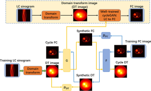
Figure 1 depicts the overall framework of the proposed method, including the training stage and prediction stage. In the training step, the FC images were used as the learning target of the corresponding LC sinograms. A CycleGAN architecture was employed to learn the mapping between FC images and DT images, where the DT images are obtained by the LC sinograms through the DT layer. This DT layer employs a back-projection operation that converts LC sinogram data into image domains (LC→DT). By introducing target mapping (DT images to FC images) and inverse mapping (FC images to DT images), the CycleGAN architecture treats the transformation as a closed loop. The network structure of the algorithm is described in detail in the next section.

Figure 1 Schematic flow chart of the proposed LCPR-Net in the CycleGAN framework for LC sinogram data reconstruction. LCPR-Net, low-count positron emission tomography image reconstruction network; CycleGAN, cycle-consistent generative adversarial network.

Network architecture

Generative network

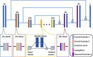
Figure 2 shows the detailed network structure of the generator of the proposed LC PET image reconstruction network (LCPR-Net) method. The generator uses a U-shaped network consisting of an encoding part, a transformation part, a decoding part, and skip connections. The size of all the convolution kernels used is 3×3. The encoding part consists of six convolution-instance norm (IN)-leaky rectified linear unit (Leaky ReLU) (CIL) blocks (convolution, IN and Leaky ReLU activation functions). The dimension of the image is reduced by half by setting the step size of the convolution to 2, and the number of feature maps is expanded by setting the number of convolution kernels to 2. In the transformation part, we use five residual block modules to implement generator learning. The decoding part consists of two deconvolution-IN-Leaky ReLU (DIL) blocks (deconvolution, IN and Leaky ReLU activation functions) and four CIL blocks. The DIL blocks consist of a deconvolution function with a stride of 2, the IN function, and the Leaky ReLU activation function. Among them, a deconvolution function with a stride of 2 expands the image dimension by a factor of 2 while reducing the number of feature maps by half. The final layer sets the number of convolution kernels to 1 as the output of the network. To solve the loss of image detail and network training problems caused by overly deep convolutional layers, we introduce long skip connections between the encoder and decoder parts.

Figure 2 The generator of the proposed LCPR-Net. LCPR-Net, low-count positron emission tomography image reconstruction network.

Discriminative network

In Figure 3, reference is made to recent successful applications of GANs (42). The discriminator D is composed of eight convolutional layers and two fully connected layers. Each convolutional layer is followed by IN and Leaky ReLU activation functions. After the convolutional layer, we added two dense layers. The first fully connected layer has 1,024 units and is followed by a Leaky ReLU activation function. Because we use the least-squares loss to measure the difference between the generated image and the real image, we remove the sigmoid activation layer, so the other fully connected layer has only 1 unit as the output. Similar to the generator, the size of all the convolution kernels used is 3×3, and the number of convolution kernels in each layer is 32, 32, 64, 64, 128, 128, 256, and 256.

Figure 3 The discriminator of the proposed method.

Loss function

Adversarial loss

In the original GAN, G attempts to produce G(x), and D distinguishes the generated images G(x) and the target images y with a binary label. The loss function is defined as:

$$mi{n}_{G}ma{x}_D\left(D,G\right)={\mathbb{E}}_{x~p_{data}\left(x\right)}\left[logD\left(x\right)\right]+{\mathbb{E}}_{y~p_y\left(y\right)}\left[\text{log}\left(1-D\left(G\left(y\right)\right)\right)\right]$$[1]

However, this logarithmic form makes training and convergence difficult, as it can cause vanishing gradient problems. Therefore, we apply the least-squares loss used in least-squares GANs (LSGANs) (43) in the original CycleGAN model to solve this problem. We use generators G and F for domain conversion between the DT and FC images, G: DT→FC and F: FC→DT. For the discriminator, the purpose of D_DT is to distinguish between a real DT image and a synthesized fake image G(x), and the purpose of D_FC is to distinguish between a real FC image and a synthesized fake image F(y). For the reference domain X, which is the DT image domain, the loss is defined by:

$$mi{n}_D{V}_{LSGAN}\left(D_{DT}\right)={\mathbb{E}}_{x~p_x\left(x\right)}\left[{\left(D_{DT}\left(x\right)-1\right)}^2\right]+{\mathbb{E}}_{y~p_y\left(y\right)}\left[{\left(D_{DT}\left(F\left(y\right)\right)\right)}^2\right]$$[2]

$$mi{n}_G{V}_{LSGAN}\left(G\right)={\mathbb{E}}_{y~p_y\left(y\right)}\left[{\left(D_{DT}\left(F\left(y\right)\right)-1\right)}^2\right]$$[3]

For the target domain Y, which is the FC image domain, the loss is:

$$mi{n}_D{V}_{LSGAN}\left(D_{FC}\right)={\mathbb{E}}_{y~p_y\left(y\right)}\left[{\left(D_{FC}\left(y\right)-1\right)}^2\right]+{\mathbb{E}}_{x~p_x\left(x\right)}\left[{\left(D_{FC}\left(G\left(x\right)\right)\right)}^2\right]$$[4]

$$mi{n}_G{V}_{LSGAN}\left(F\right)={\mathbb{E}}_{x~p_x\left(x\right)}\left[{\left(D_{FC}\left(G\left(x\right)\right)-1\right)}^2\right]$$[5]

where G and F are generators that generate the FC image and DT image, respectively. D_DT is the discriminator that distinguishes between a DT image and a synthetic DT image. D_FC is the discriminator that distinguishes between an FC image and a synthetic FC image.

Cycle consistency loss

In a cyclic framework, to enhance the mapping relationship, the cyclic consistency loss can be expressed as:

$$L_{CYC}\left(G,F\right)={\mathbb{E}}_x\left[F{\left(G\left(x)\right)-x\right)}_2\right]+{\mathbb{E}}_y\left[G\left(F\left(y\right)\right)-y_2\right]$$[6]

where F(G(x))≈x represents forward cycle consistency, G(F(y))≈y represents backward cycle consistency, and ${\Vert ·\Vert }_2$ denotes theL₂ norm. This cycle consistency loss prevents the degradation of adversarial learning.

Supervised loss

In this study, we have paired data, so we can train the model in a supervised way and define the supervised loss function as:

$$L_{SUP}\left(G,F\right)={\mathbb{E}}_{x,y}\left[G\left(x\right)-y{)}_2\right]+{\mathbb{E}}_{x,y}\left[F\left(y\right)-x_2\right]$$[7]

where G(x) is an image close to y generated by source image x through generator G and F(y) is an image close to x generated by source image y through generator F. We can then define the final loss by:

$$L_{total}=L_{LSGAN}\left(D_{DT},G\right)+L_{LSGAN}\left(D_{FC},F\right)+{\lambda }_1{L}_{CYC}\left(G,F\right)+{\lambda }_2{L}_{SUP}\left(G,F\right)$$[8]

where λ₁ and λ₂ are parameters for balancing among different penalties and we empirically set them both to 1.

Implementation details

In the proposed LCPR-Net, we use the Xavier initializer to initialize the weights of the convolutional layer (44). Based on the computer hardware used, the training batch size is set to 4. Because the batch size is small, instance normalization (45) is used after each convolutional layer instead of batch normalization. All the Leaky ReLU activation functions used have a slope of α=0.2. During the experiment, we empirically set λ₁=1 and λ₂=1 in the loss function. In the proposed network, we use the Adam optimizer to optimize the loss function with a learning rate of 0.00001, β₁=0.5, and β₂=0.99. All the experiments were performed on a PC equipped with an NVIDIA GeForce GTX 1080Ti GPU using the TensorFlow library.

Experiment and validation

In this study, we used hospital patient data to verify the feasibility of the proposed method. The performance of the proposed LCPR-Net is quantitatively evaluated using two evaluation indicators: the peak signal-to-noise ratio (PSNR) and the mean squared error (MSE).

Simulation study

Clinical PET image data for 30 patients scanned using a GE Discovery PET/CT 690 machine were used in the study. A whole-body scan image was available for each patient, and each scan included 310 2D slices. We used data from 24 patients as the training set and data from 6 patients as the test set. The dataset was tripled in size by flipping the images left and right and rotating ±10° to avoid overfitting problems during network training. These 2D slices were then projected using system matrix forward projection to generate corresponding noise-free sinogram data. To simulate real data acquisition, 20% of real events were added to simulate random and scattered events (46). To verify the performance of the proposed LCPR-Net for different count levels, we normalized the simulated sinogram data to 5 M, 500 K, and 50 K counts to represent different doses. Finally, independent Poisson noise was introduced 20 times in the sinogram data to simulate real noise data.

Evaluation methods

To verify the performance of the proposed LCPR-Net, four algorithms are used for comparison [expectation-maximization (EM) reconstruction plus post-Gaussian filtering, EM reconstruction plus NLM denoising, a CNN and a GAN]. To ensure the fairness of the experiment, the network structure of the CNN is the same as that of the generator used in the LCPR-Net proposed in this paper. The network structure of the GAN is shown in Figure 4, where G represents the generator of the network and D_FC represents the discriminator of the network. They have the same structure as G and D_FC of the proposed LCPR-Net. Among them, the loss function of the CNN is the MSE loss, and the parameter is set to 1. The loss function of the GAN is the MSE and the discriminator losses, and their parameter settings correspond to that of the LCPR-Net and are both set to 1.

Figure 4 Schematic flow chart of the GAN framework for LC sinogram data reconstruction. GAN, generative adversarial network; LC, low-count.

Quantitative analysis

To evaluate the performance of the proposed LCPR-Net, we use three evaluation indicators to verify the reconstruction results. The first indicator is the structural similarity index (SSIM) (47), which is used for visual image quality assessment and takes into account the overall structure of the image. The value of this index ranges from 0–1, and the higher the value is, the closer the image structure is to that of the real image. We use the PSNR as the second metric, where higher values indicate better image quality:

$$PSNR=10lo{g}_{10}\left(\frac{ma{x}^2}{ \frac{1}{n}{{\displaystyle \sum }}_{i=1}^n{\left(x_i-y_i\right)}^2}\right)$$[9]

The third evaluation metric is the relative root mean square error (rRMSE), where lower values indicate better image quality:

$$rRMSE=\frac{\sqrt{ \frac{1}{n}{{\displaystyle \sum }}_{i=1}^n{\left(x_i-y_i\right)}^2}}{\overline{y}}$$[10]

where x_i and y_i are the pixel values of the reconstructed image and the real image, respectively, n is the number of pixel values of the image, $\overline{y}$ is the average pixel value of the real image and max represents the maximum value of the image pixels.

Results

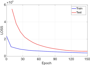
Figure 5 shows the convergence of the loss curve of the training set and the validation set during the training process of the LCPR-Net. When the network training process reaches 150 epochs, the loss curve of the verification set no longer decreases, so to avoid network overfitting, we stop training.

Figure 5 The convergence curve of the loss curve between the reconstructed image and the real image. The loss curve of the training set is shown in blue, and the loss curve of the test set is shown in red. The test set loss curve stops decreasing at approximately 150 epochs.

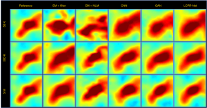
In this study, we discuss the reconstruction performance of the proposed LCPR-Net based on LC sinogram data. We compare the results of EM reconstruction plus post-Gaussian filtering, EM reconstruction plus NLM denoising, CNN reconstruction and GAN reconstruction with the results of the proposed LCPR-Net. In addition, the PSNR, SSIM and rRMSE are used for the quantitative evaluation of the images. We selected three representative slices, and the reconstruction results using different methods are shown in Figure 6. All the reconstructed images are for 500 K counts. The first column is the real image. The second, third, fourth, fifth and last columns are the results generated by the EM algorithm plus post-Gaussian filtering, the EM algorithm plus NLM denoising, the CNN, the GAN, and the proposed LCPR-Net. As indicated by the red arrow, the image reconstructed by using LCPR-Net is closest to the real image, and it is worth noting that because the GAN optimizes the objective functions individually, it generates features that do not appear in the target image. Additionally, the LCPR-Net cyclically optimizes the objective function to avoid this problem. To further verify the performance of the LCPR-Net, we calculated the PSNR, SSIM and rRMSE for the methods shown in Figure 6 and listed the results in Table 1. We can see that at 500 K counts, the PSNR and SSIM values of the image reconstructed by the LCPR-Net are the highest and the rRMSE value is the smallest. In addition, Figure 7 shows the profiles of the reconstructed images using different methods along the red line of the three positions shown in slices one, two and three in Figure 6. The images reconstructed by our LCPR-Net are closer to the reference images than those reconstructed by the other methods.

Figure 6 Three slices of one patient reconstructed for 500 K counts using the different methods.

Table 1 Quantitative evaluation of the different methods for the different slices in Figure 7
Full table

Figure 7 Profiles of the three positions along the red lines in Figure 6.

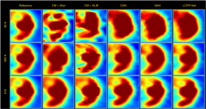
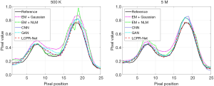
To compare the performance of LCPR-Net at different counts, we selected one of the slices to analyze the reconstructed images for 5 M, 500 K, and 50 K counts. Figure 8 shows the reconstructed images of selected slices for different counts and with different methods. To compare the image details, we enlarged the region of interest (ROI) in Figure 8, as shown in Figures 9,10. These images are located in the corresponding red boxes in Figure 8. We find that for 50 K and 500 K counts, the reconstruction results of the three deep learning methods are significantly better than those of the traditional EM algorithm plus Gaussian filtering and the EM algorithm plus NLM denoising, and the proposed LCPR-Net outperforms the CNN and GAN in image detail retention. In the case of the 5 M counts, the results of our method are slightly better than those of the other two methods. The PSNR, SSIM and rRMSE of the whole image are listed in Table 2, and two red rectangular regions in Figure 8 are presented in Tables 3,4. As shown in Tables 2,3,4, the proposed LCPR-Net method has the highest PSNR and SSIM values and the smallest rRMSE value. Figure 11 shows the profile of the slice in Figure 8 for 500 K and 5 M counts using three different methods to reconstruct the image at three positions along the red line in Figure 8 for 500 K and 5 M counts. We can see that the images reconstructed by LCPR-Net are closer to the reference images, which indicates that LCPR-Net achieves a better reconstruction performance in the case of LC sinogram data than the other state-of-the-art methods.

Figure 8 Images reconstructed using the different methods for 50 K, 500 K and 5 M counts.

Figure 9 The first zoomed-in ROI is marked by the red rectangle in Figure 8. ROI, region of interest.

Figure 10 The second zoomed-in ROI is marked by the red rectangle in Figure 8. ROI, region of interest.

Table 2 Quantitative evaluation of the results of the different methods from Figure 8 for 50 K, 500 K, and 5 M counts
Full table

Table 3 Quantitative evaluation of the results of the different methods from Figure 9 for 50 K, 500 K, and 5 M counts
Full table

Table 4 Quantitative evaluation of the results of the different methods from Figure 10 for 50 K, 500 K, and 5 M counts
Full table

Figure 11 Profiles of the two positions along the red lines in Figure 8.

Discussion

In this work, we proposed LCPR-Net, which uses a CycleGAN to reconstruct high-quality FC PET images from LC PET sinograms. Although the traditional GAN provides excellent performance for reconstructed images (48), there are still two important shortcomings of this approach. First, due to the degradation of the mapping process, the GAN method will generate features that are not present in the target images (41). Second, the model will collapse due to optimizing the adversarial objectives individually (38). To solve these problems, a CycleGAN is designed to constrain the generator by introducing an inverse transform in a cyclic manner. The results indicate that the CycleGAN performs better in LC PET reconstruction problems than GANs.

Through an analysis of the above experimental results, the images reconstructed by the two deep learning methods for 500 K and 50 K counts are significantly better than the images obtained by traditional iterative reconstruction. The reconstructed image for the 5 M count is visually similar to that based on traditional iterative reconstruction, but the quantitative analysis results indicate that the proposed method yielded higher PSNR and SSIM values and smaller rRMSE values. In addition, due to the cyclic consistency introduced by the proposed LCPR-Net, compared with GAN reconstruction, LCPR-Net eliminates the potential risk that the network may yield features that are not present in the target images due to the degeneracy of the mapping process. In the quantitative results, LCPR-Net has higher PSNR and SSIM values than the GANs.

The proposed LCPR-Net has the following main advantages. First, an LC PET sinogram is directly reconstructed to obtain an FC PET image. Second, reconstructing images under the CycleGAN framework yields better results than reconstruction based on separately optimized GANs. Third, compared with the traditional model-based iterative reconstruction approach, the reconstruction time of the proposed method is faster without the use of a system matrix.

This work still has some limitations. First, because the training data are simulation data, actual clinical data cannot be fully simulated. This problem can be alleviated by using a complete Monte Carlo simulation model [such as the Geant4 application for tomographic emission (GATE)], which can provide highly accurate sinogram data. Second, we were unable to reconstruct a real PET image due to the lack of real scan data, but we reconstructed the LC sinogram data of simulated clinical patients and obtained good results. Third, the proposed LCPR-Net is based on the reconstruction of 2D space, which lacks the characteristics of spatial data. Therefore, our future work will consider the reconstruction of 3D sinogram data. Our method back-projects a large number of sinograms into one single 3D back-projected image, so we have fewer issues with memory than conventional fully 3D reconstruction methods that operate on the fully 3D set of sinograms. Finally, although the proposed method outperforms other state-of-the-art methods, the reconstructed image still differs slightly from the real image.

Conclusions

We proposed a cycle-consistent least-squares regression adversarial training framework for reconstructing PET images from LC sinogram data. This approach can provide doctors with high-quality PET images and reduce the injected radiotracer dose and scanning time. The quantitative experimental results indicate that the proposed LCPR-Net outperforms the traditional EM algorithm with Gaussian postfiltering method and the GAN-based reconstruction method.

Acknowledgments

The authors would like to thank the editor and anonymous reviewers for their constructive comments and suggestions.

Funding: This work was supported by the Guangdong Special Support Program of China (2017TQ04R395), the National Natural Science Foundation of China (81871441, 91959119), the Shenzhen International Cooperation Research Project of China (GJHZ20180928115824168), the Guangdong International Science and Technology Cooperation Project of China (2018A050506064), the Natural Science Foundation of Guangdong Province in China (2020A1515010733), and the Fundamental Research Funds for the Central Universities (N2019006, N180719020).

Footnote

Conflicts of Interest: All authors have completed the ICMJE uniform disclosure form (available at http://dx.doi.org/10.21037/qims-20-66). Dr. DL serves as an unpaid editorial board member of Quantitative Imaging in Medicine and Surgery. The other authors have no conflicts of interest to declare.

Ethical Statement: The study was approved by the Tongji Hospital, Tongji Medical College, Huazhong University of Science and Technology, and informed consent was obtained from all the patients.

Open Access Statement: This is an Open Access article distributed in accordance with the Creative Commons Attribution-NonCommercial-NoDerivs 4.0 International License (CC BY-NC-ND 4.0), which permits the non-commercial replication and distribution of the article with the strict proviso that no changes or edits are made and the original work is properly cited (including links to both the formal publication through the relevant DOI and the license). See: https://creativecommons.org/licenses/by-nc-nd/4.0/.

References

1. Beyer T, Townsend DW, Brun T, Kinahan PE, Charron M, Roddy R, Jerin J, Young J, Byars L, Nutt R. A combined pet/ct scanner for clinical oncology. J Nucl Med 2000;41:1369-79. [PubMed]
2. Machac J. Cardiac positron emission tomography imaging. Semin Nucl Med 2005;35:17-36. [Crossref] [PubMed]
3. Gunn RN, Slifstein M, Searle GE, Price JC. Quantitative imaging of protein targets in the human brain with PET. Phys Med Biol 2015;60:R363-411. [Crossref] [PubMed]
4. Hutchins GD, Rogers WL, Chiao P, Raylman RR, Murphy BW. Constrained least squares filtering in high resolution PET and SPECT imaging. IEEE Trans Nucl Sci 1990;37:647-51. [Crossref]
5. Hashimoto F, Ohba H, Ote K, Tsukada H. Denoising of Dynamic Sinogram by Image Guided Filtering for Positron Emission Tomography. IEEE Trans Radiat Plasma Med Sci 2018;2:541-8. [Crossref]
6. Peltonen S, Tuna U, Sanchez-Monge E, Ruotsalainen U (eds). PET sinogram denoising by block-matching and 3D filtering. Valencia, Spain: Nuclear Science Symposium & Medical Imaging Conference, 2011.
7. Bian Z, Huang J, Ma J, Lu L, Niu S, Zeng D, Feng Q, Chen W. Dynamic Positron Emission Tomography Image Restoration via a Kinetics-Induced Bilateral Filter. PLoS One 2014;9:e89282. [Crossref] [PubMed]
8. Shepp LA, Vardi Y. Maximum likelihood reconstruction for emission tomography. IEEE Trans Med Imaging 1982;1:113-22. [Crossref] [PubMed]
9. Zhou J, Coatrieux JL, Bousse A, Shu H, Luo L. A Bayesian MAP-EM algorithm for PET image reconstruction using wavelet transform. IEEE Trans Nucl Sci 2007;54:1660-9. [Crossref]
10. Hudson HM, Larkin RS. Accelerated image reconstruction using ordered subsets of projection data. IEEE Trans Med Imaging 1994;13:601-9. [Crossref] [PubMed]
11. Zeng T, Gao J, Gao D, Kuang Z, Sang Z, Wang X, Hu L, Chen Q, Chu X, Liang D. A GPU-accelerated fully 3D OSEM image reconstruction for a high-resolution small animal PET scanner using dual-ended readout detectors. Phys Med Biol 2020. Epub ahead of print. [Crossref] [PubMed]
12. Dutta J, Leahy RM, Li Q. Non-Local Means Denoising of Dynamic PET Images. PLoS One 2013;8:e81390. [Crossref] [PubMed]
13. Tang J, Yang B, Wang Y, Ying L. Sparsity-constrained PET image reconstruction with learned dictionaries. Phys Med Biol 2016;61:6347-68. [Crossref] [PubMed]
14. Cong Y, Zhang S, Lian Y (eds). K-SVD Dictionary Learning and Image Reconstruction Based on Variance of Image Patches. Hangzhou, China: 8th International Symposium on Computational Intelligence and Design (ISCID), 2015.
15. Xu Q, Yu H, Mou X, Zhang L, Hsieh J, Wang G. Low-dose X-ray CT reconstruction via dictionary learning. IEEE Trans Med Imaging 2012;31:1682-97. [Crossref] [PubMed]
16. Zhang W, Gao J, Yang Y, Liang D, Liu X, Zheng H, Hu Z. Image reconstruction for positron emission tomography based on patch‐based regularization and dictionary learning. Med Phys 2019;46:5014-26. [Crossref] [PubMed]
17. Yu X, Wang C, Hu H, Liu H, Li Z. Low Dose PET Image Reconstruction with Total Variation Using Alternating Direction Method. PLoS One 2016;11:e0166871. [Crossref] [PubMed]
18. Wang C, Hu Z, Shi P, Liu H (eds). Low dose PET reconstruction with total variation regularization. Chicago, IL: 36th Annual International Conference of the IEEE Engineering in Medicine and Biology Society, 2014:1917-20.
19. Tian Z, Jia X, Yuan K, Pan T, Jiang SB. Low-dose CT reconstruction via edge-preserving total variation regularization. Phys Med Biol 2011;56:5949-67. [Crossref] [PubMed]
20. Chen Y, Yin FF, Zhang Y, Zhang Y, Ren L. Low dose cone-beam computed tomography reconstruction via hybrid prior contour based total variation regularization (hybrid-PCTV). Quant Imaging Med Surg 2019;9:1214. [Crossref] [PubMed]
21. Chan C, Fulton R, Barnett R, Feng DD, Meikle S. Postreconstruction Nonlocal Means Filtering of Whole-Body PET With an Anatomical Prior. IEEE Trans Med Imaging 2014;33:636-50. [Crossref] [PubMed]
22. Zhang H, Ma J, Wang J, Liu Y, Han H, Lu H, Moore W, Liang Z. Statistical image reconstruction for low-dose CT using nonlocal means-based regularization. Part II: An adaptive approach. Comput Med Imaging Graph 2015;43:26-35. [Crossref] [PubMed]
23. Fumene Feruglio P, Vinegoni C, Gros J, Sbarbati A, Weissleder R. Block matching 3D random noise filtering for absorption optical projection tomography. Phys Med Biol 2010;55:5401-15. [Crossref] [PubMed]
24. Wang G. A Perspective on Deep Imaging. IEEE Access 2016;4:8914-24.
25. Xu J, Gong E, Pauly J, Zaharchuk G. 200x Low-dose PET Reconstruction using Deep Learning. arXiv e-prints 2017. Available online: https://arxiv.org/abs/1712.04119
26. Gong K, Guan J, Liu CC, Qi J. PET Image Denoising Using a Deep Neural Network Through Fine Tuning. IEEE Trans Radiat Plasma Med Sci 2019;3:153-61. [Crossref] [PubMed]
27. Hu Z, Li Y, Zou S, Xue H, Sang Z, Liu X, Yang Y, Zhu X, Liang D, Zheng H. Obtaining PET/CT images from non-attenuation corrected PET images in a single PET system using Wasserstein generative adversarial networks. Phys Med Biol 2020;65:215010. [Crossref] [PubMed]
28. Zhang Q, Zhang N, Liu X, Zheng H, Liang D. PET Image Reconstruction Using a Cascading Back-Projection Neural Network. IEEE J Sel Top Signal Process 2020;14:1100-11. [Crossref]
29. Hu Z, Xue H, Zhang Q, Gao J, Zhang N, Zou S, Teng Y, Liu X, Yang Y, Liang D. DPIR-Net: Direct PET image reconstruction based on the Wasserstein generative adversarial network. IEEE Trans Radiat Plasma Med Sci 2020. Epub ahead of print. [Crossref]
30. Gong K, Guan J, Kyungsang K, Xuezhu Z, Jaewon Y, Youngho S, El Fakhri G, Jinyi Q, Quanzheng L. Iterative PET Image Reconstruction Using Convolutional Neural Network Representation. IEEE Trans Med Imaging 2019;38:675-85. [Crossref] [PubMed]
31. Cai S, Tian Y, Lui H, Zeng H, Wu Y, Chen G. Dense-UNet: a novel multiphoton in vivo cellular image segmentation model based on a convolutional neural network. Quant Imaging Med Surg 2020;10:1275. [Crossref] [PubMed]
32. Zhu B, Liu JZ, Cauley SF, Rosen BR, Rosen MS. Image reconstruction by domain-transform manifold learning. Nature 2018;555:487-92. [Crossref] [PubMed]
33. Häggström I, Schmidtlein CR, Campanella G, Fuchs TJ. DeepPET: A deep encoder-decoder network for directly solving the PET image reconstruction inverse problem. Med Image Anal 2019;54:253-62. [Crossref] [PubMed]
34. Goodfellow IJ, Pouget-Abadie J, Mirza M, Xu B, David Warde-Farley, Ozair S, Courville A, Bengio Y. Generative adversarial networks. Available online: https://papers.nips.cc/paper/5423-generative-adversarial-nets.pdf
35. Wang Y, Yu B, Wang L, Zu C, Lalush DS, Lin W, Wu X, Zhou J, Shen D, Zhou L. 3D conditional generative adversarial networks for high-quality PET image estimation at low dose. NeuroImage 2018;174:550-62. [Crossref] [PubMed]
36. Wolterink JM, Leiner T, Viergever MA, Isgum I. Generative Adversarial Networks for Noise Reduction in Low-Dose CT. IEEE Trans Med Imaging 2017;36:2536-45. [Crossref] [PubMed]
37. Yang G, Yu SM, Dong H, Slabaugh G, Dragotti PL, Ye XJ, Liu FD, Arridge S, Keegan J, Guo YK, Firmin D. DAGAN: Deep De-Aliasing Generative Adversarial Networks for Fast Compressed Sensing MRI Reconstruction. IEEE Trans Med Imaging 2018;37:1310-21. [Crossref] [PubMed]
38. You C, Li G, Zhang Y, Zhang X, Shan H, Li M, Ju S, Zhao Z, Zhang Z, Cong W, Vannier MW, Saha PK, Hoffman EA, Wang G. CT super-resolution GAN constrained by the identical, residual, and cycle learning ensemble (GAN-circle). IEEE Trans Med Imaging 2019. Available online: https://arxiv.org/abs/1808.04256
39. Goodfellow I. NIPS 2016 Tutorial: Generative Adversarial Networks. Available online: https://arxiv.org/abs/1701.00160
40. Zhu JY, Park T, Isola P, Efros AA. Unpaired Image-to-Image Translation using Cycle-Consistent Adversarial Networks. 2018. Available online: https://arxiv.org/abs/1703.10593
41. Kang E, Koo HJ, Yang DH, Seo JB, Ye JC. Cycle-consistent adversarial denoising network for multiphase coronary CT angiography. Med Phys 2019;46:550-62. [Crossref] [PubMed]
42. Hu Z, Jiang C, Sun F, Zhang Q, Ge Y, Yang Y, Liu X, Zheng H, Liang D. Artifact correction in low-dose dental CT imaging using Wasserstein generative adversarial networks. Med Phys 2019;46:1686-96. [Crossref] [PubMed]
43. Mao X, Li Q, Xie H, Lau RYK, Wang Z, Smolley SP. Least squares generative adversarial networks. Available online: https://arxiv.org/abs/1611.04076
44. Glorot X, Bengio Y. Understanding the difficulty of training deep feed forward neural networks. Proceedings of the Thirteenth International Conference on Artificial Intelligence and Statistics, 2010. Available online: http://proceedings.mlr.press/v9/glorot10a/glorot10a.pdf
45. Ulyanov D, Vedaldi A. Instance normalization: The missing ingredient for fast stylization. Available online: https://arxiv.org/abs/1607.08022
46. Mawlawi O, Podoloff DA, Kohlmyer S, Williams JJ, Stearns CW, Culp RF, Macapinlac H. Performance characteristics of a newly developed PET/CT scanner using NEMA standards in 2D and 3D modes. J Nucl Med 2004;45:1734-42. [PubMed]
47. Wang Z, Bovik AC, Sheikh HR, Simoncelli EP. Image quality assessment: from error visibility to structural similarity. IEEE Trans Image Process 2004;13:600-12. [Crossref] [PubMed]
48. Nie D, Trullo R, Lian J, Wang L, Petitjean C, Ruan S, Wang Q, Shen D. Medical Image Synthesis with Deep Convolutional Adversarial Networks. IEEE Trans Biomed Eng 2018;65:2720-30. [Crossref] [PubMed]