Evaluation of magnetic resonance image segmentation in brain low-grade gliomas using support vector machine and convolutional neural network
Introduction
Glioma is a type of tumor account for approximately 30% of all brain and central nervous system tumors and 80% of all malignant brain tumors (1). Low-grade gliomas (LGG) are a group of WHO grade II and grade III brain tumors and tend to evolve to higher grade glioma (2). Magnetic resonance imaging (MRI) is a promising non-invasive imaging technique for brain structural mapping and analysis. MRI can be implemented to detect brain tumors including gliomas due to its ability to generate unique soft-tissue contrast and high image resolution in humans (3).
Brain tumor segmentation is to extract the specified clinical information and diagnostic features from brain tumor images by separating the tumor from other normal brain tissues (4,5). The information extracted by segmentation plays an important role in diagnosis, staging and treatment (6). Based on MRI’s property, segmentation of MRI LGG images could benefit significantly to clinical diagnosis and research.
Artificial intelligence (AI) technology has demonstrated a tremendous success in MR imaging reconstruction and analysis (7,8). In the application of MR image segmentation, AI can be used to implement automatic image segmentation and significantly improve the efficiency of image processing and analysis. Machine learning is a subset of AI technology coined in 1959 by Arthur Samuel (9,10). It is an algorithm which solves the problem by learning through experience and improves itself without human intervention (11). Machine learning is widely applied in analyzing MRI brain tumor images, including normal (e.g., white matter and gray matter) and abnormal (e.g., brain tumors) brain tissue segmentation (3). Based on morphological differences between normal and abnormal tissues illustrated in MR images, machine learning algorithms can be set to perform LGG segmentation automatically.
Based on the utilization of labels of a dataset, machine learning can be classified into different categories as supervised learning, semi-supervised learning, and unsupervised learning (12,13). In supervised learning, all samples are combined with two parts: input observations (features) and output observations (labels) (9). In unsupervised learning, all samples have only one set of observations or features and possess no labels. Therefore, the system will try to find out relations between all samples and to cluster samples in the same class together by itself (13). Semi-supervised learning is a combination of supervised learning and unsupervised learning, which uses both labeled and unlabeled data for training (14). In this study, all the image data obtained have the corresponding mask, which can be considered as labels. Therefore, all work presented in this paper will be focused on supervised learning.
There have been several machine learning algorithms. Machine learning algorithms are widely applied for MRI brain tumor segmentation, such as Bayes, Random Forest, k-means, support vector machine (SVM), and artificial neural networks (ANNs). Based on the model structure, machine learning can be divided into traditional machine learning and deep learning.
Traditional machine learning models are generally mathematical algorithms such as linear regression trained based on manually organized features; while a deep learning model is a combination of several connected neurons learning directly from raw data (11).
SVMs are advanced traditional machine learning algorithms for binary and non-linear problems. With the ability to transfer non-linear problem to linear, SVM demonstrated its advantages in MR image segmentation applications (15).
Deep learning is a special subset of machine learning. In deep learning, the model of ANNs is used. ANNs are the basic systems of deep learning and they operate as a simplified model of the human brain (16). Convolutional Neural Network (CNN) is a type of ANNs, which is specified to solve image processing and analysis problems. CNN is also widely applied to medical image research due to its robust performance (17).
As for brain LGG segmentation of MR images, SVM and CNN perform differently. In this work, we will first develop the SVM and CNN models to solve the LGG MRI segmentation problems, and then compare and analyze the performance of two models quantitatively. The results of this study could provide model selection suggestions for LGG MR image segmentation problems.
Methods
Dataset
The dataset used in this work contains MR images obtained from The Cancer Imaging Archive (TCIA) (https://wiki.cancerimagingarchive.net/display/Public/TCGA-LGG) together with manual fluid-attenuated inversion recovery (FLAIR) abnormality segmentation masks. Images correspond to 109 patients included in The Cancer Genome Atlas (TCGA) LGG collection (https://www.cancer.gov/about-nci/organization/ccg/research/structural-genomics/tcga) with at least FLAIR sequence and genomic cluster data available. Each patient has over 20 pairs of images and corresponding mask data. The dataset is open source and free to download (https://www.kaggle.com/mateuszbuda/lgg-mri-segmentation#TCGA_CS_4943_20000902_11_mask.tif). Each MR image is an RGB three-channel image with 256×256 pixels in each channel. Each image also has a corresponding mask image with the same size but only one channel. Figure 1 shows two pairs of images and masks from two patients.

In this data set, some MR images with less information, such as only black images without clear brain anatomic structures, are removed manually to prune the data set to make it perform better in training. Finally, 2,470 MRI and mask image pairs are selected to make up the dataset.
SVM
SVM is a strong supervised machine learning model for binary and non-linear classification problems based on the Statistical Learning Theory (15).
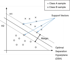
Founded in An Introduction to Support Vector Machines and Other Kernel-based Learning Methods (18) and Guo et al.’s research (19), SVM constructs a hyperplane called the optimal separation hyperplane (OSH) in the feature space to separate the two classes and retain the maximum margin between the two classes, thereby achieving binary classification. Assume there is a data set
Algebraically, the classification problem is set as:
[1]
A loose variable
[2]
Resolving Eq. [2] requires solving the quadratic programming (QP) problem (20), which is described as:
[3]
In the QP problem, ai is Lagrange multipliers. All coefficients ai that are not 0 are marked as
[4]
[5]
NSV is the number of SVs and
[6]
As the classifier function is shown, solving the QP problems is the key to train SVM.
For non-linear problems, the original input set of variables x needs to be projected to a higher dimension space and the kernels are implemented. A kernel is a function K with project Φ:
[7]
So, the SVM with the kernel is defined as:
[8]
Gaussian kernel {Eq. [9]} is a widely used kernel in non-linear problems due to its properties that affect less to the points distant from separation boundary (15). In Eq. [9], u and v are points in feature space and K (u,v) is Gaussian similarity of u and v. By applying a Gaussian kernel, new features of a point are created as Gaussian similarities of the point and all SVs in the original feature space, in order to achieve the transformation of nonlinear to linear problems.
[9]
CNN
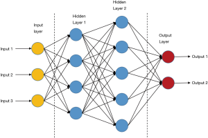
ANNs are the basis of deep learning. It is a kind of computing systems with neural structures similar to biological brains (16). ANNs are composed of connected units or nodes called artificial neurons, which are similar to biological neurons. Data enter the ANN system with an input layer, are then calculated by one or more subsequent hidden layers, and finally end at an output layer, which represents the prediction or result (as shown in Figure 3). In the ANNs architecture, every connection of two neurons is assigned a weight that represents the weighing of input neuron on output neuron. One neuron can have more than one input or output connections (21). The input to a neuron is computed by a weighted sum of its former layer outputs and connection weights. For example, an input layer is written as a i×1 matrix Ii, in which i is the number of inputs, while the output layer h1 has j neurons and is written as a j×1 matrix
The training of an ANN is to make predictions as close to real outputs as possible by adjusting weights and other parameters in the network to improve the accuracy which can be observed as reducing the training error. Training error is measured by a function called loss function or cost function (11). In binary classification, cross-entropy is usually used as loss function {Eq. [10]}, in which y is real condition and p is predicted condition. Backpropagation (BP) is a primary used algorithm in training ANNs for supervised learning. BP uses the chain rules to compute the gradient of the cost function with respect to every weight and adjusts weights with gradient descent to reduce the loss (23). This computation will be a huge job, because an ANN usually has millions of parameters to be trained and millions of data need to be processed when passing through the layer. Therefore, a powerful computer is essential for training ANNs.
[10]
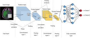
CNN is a type of ANNs specifically used for image processing problems or some other computer version field (17). CNNs consist of convolutional layers, activation layers, pooling layers, fully connected layers, an input layer, and an output layer. CNN preserves spatial relationships in the data by passing inputs through the layers that retain the original relationship of inputs data and each operation of layers operates on a small region of the previous layer (Figure 4) (11).
CNNs are widely applied to medical image segmentation problems (24-29). Fully convolutional network (FCN) is a type of CNN proposed for segmentation problems (30). A specified CNN called “U-Net” is widely used for image segmentation problem. U-Net was initially developed for biomedical image segmentation based on the FCN (28,30). The network consists of a contracting path and an expansive path, which makes its architecture to have a U-shape. The left part is the contracting path, which is a typical convolutional network, while the right part is the expansive path that consists up-convolutions and concatenations with features from the contracting path (Figure 5) (28). The spatial information is reduced while feature information is increased in the contracting path, and the spatial information will be restored in an expansive path to make sure the prediction and input have the same spatial size. The feature information is extracted by the whole network.
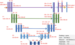
In this work, U-Net is applied as CNN for MRI brain LGG segmentation problem.
Model evaluation
It is important to evaluate the performance of a model once it gets trained. Generally, model evaluation includes accuracy, confusion matrix, precision, recall, and F1 score.
The confusion matrix is a specific 2×2 table that visualizes the performance of a machine learning model. Four cells represent the number of false positives (type I error), false negatives (type II error), true positives, and true negatives (31). Detailed information is shown in Table 1.

Full table
Accuracy is the ratio of correct predictions to total predictions, as expressed in Eq. [11]. It directly shows the classification ability of a model. However, high accuracy sometimes doesn’t mean high performance of the model if the data is unbalanced. For example, in MR image segmentation, if the image has only 1% of tumor region and the model predicts the image has no tumor, the model still achieves 99% accuracy. But it is indeed unable to classify any tumor pixels we expect.
[11]
Precision is the proportion of the true positives among all positives indicating the accuracy of model positive classification {Eq. [12]} (31).
[12]
Recall is the proportion of condition positives that are correctly classified indicating the detection sensitivity to all positives {Eq. [13]}.
[13]
F1 score is a comprehensive evaluation calculated as the harmonic average of precision and recall {Eq. [14]}. Model reaches its best with a F1 score of 1 (32).
[14]
SVM experiment
SVM model system used in this study
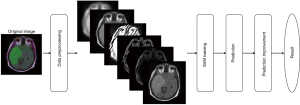
The framework of the system has 4 main steps as shown in Figure 6: (I) data preprocessing including conversion to grayscale image and feature extraction, (II) training the SVM model, (III) prediction, and (IV) prediction improvement.
Data preprocessing for SVM
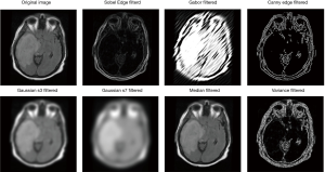
Data preprocessing includes two parts: conversion to grayscale image and feature extraction. Conversion to grayscale is using a function to convert three-channel original RGB image to one-channel 8-bit gray image. Feature extraction is the application of several spatial filters on the original grayscale image to generate multiple filtered images that can be considered as different features.
MR images are RGB images which have three channels. Conversion to grayscale images which only have one image channel can reduce the data size, thereby shortening the training time and reducing the variance. Moreover, one-channel grayscale images are also suitable for subsequent feature extraction using spatial filters.
The image segmentation model is trained to classify each pixel of the image, so each pixel is a sample. Pixels of original data have only one feature: their own original pixel values, which also means more features need to be extracted. Texture information including those detected by applying spatial filters can be considered as features (33).
After data preprocessing, several filtered images are generated as different features for following training.
Building SVM models
The initial training set was MR images of multiple patients. However, due to large differences in MR images of different patients, the training bias is high, resulting in poor model performance. In order to improve the performance of the model, only one patient’s MR image, which has 256×256 pixels and should be enough for training, is used for each model training which also means each model is only suitable for the same patient.
One MR image with clear tumor region is selected manually as the training set. To ensure the accuracy and sensitivity of the model, the sample size difference between the two classes (normal pixels, level 0 and tumor pixels, level 1) should not be too large. Usually, there are much more normal pixels than tumor pixels, so all tumor pixels are selected for the training dataset to ensure the sensitivity of the model, and twice the number of pixels are randomly selected from the normal part. In this example, the class 1 set has 5,936 pixel samples and the class 0 has 10,872 pixel samples.
Scikit-learn, a machine learning library in Python, is used to build the model. Seventy percent of pixels in both classes are chosen randomly for the training set and the rest of them are test set. It took a few seconds to train the SVM model on Google Colab cloud server with powerful CPUs and GPUs.
SVM prediction improvement
Other MR images with tumors from the same patient are used to make the prediction. Each image needs the same preprocessing as the image used for training to ensure that they have the same feature channels before prediction.
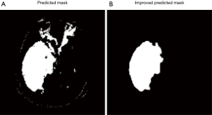
All pixels that classified by model as tumor pixels are marked as class 1. Because of misclassification, the prediction mask images usually have several pieces of masks and also some small holes inside the masks. Assuming there is only one tumor region in each image, we need to remove all small pieces and filling holes, which will significantly improve the result (Figure 7).
CNN experiment
Data augmentation for CNN
Training a CNN requires a big dataset. Small dataset will cause overfitting, which means model will only memorize the training data, suppressing the ability of CNN to generalize to unseen invariant data (34,35). Data Augmentation is a method that artificially inflates the dataset size without obtaining more data by using some transformations on original images such as dropping, padding, rotating, and horizontal flipping (34,36). In this work, the total number of MR images is 2,746, which is far from enough to prevent overfitting. In this study, all images in the training set are flipped horizontally, and then the original image and the flipped image are rotated by 90, 180, and 270 degrees, consequently expanding the training set by 8 times. All masks are flipped and rotated in the same way to their corresponding images.
The initial training set consists of 2,470 MR image pairs (90%) randomly picked and the other 276 pairs (10%) are used as test set to make sure there are enough data for each set. After augmentation, the training set was expanded by 8 times to reach 19,760, which is reasonably large for this study.
Building CNN architecture
The U-Net architecture was built in Keras library in Python. The U-Net architecture used in this work is shown in Figure 5. It has input with 256×256×3 pixels, which makes the minimum resolution of 16×16, because each one of four pooling layers reduces them by twice. Spatial resolutions of all layers are shown in Figure 5. Activation functions in all convolutional layers are set as rectified linear unit (ReLUs) (37), defined as
All filter kernels are 3×3. Parameters in each layer are initialized with the initialization algorithm by He et al. (39). 1,941,105 parameters in total need to be trained in this U-Net network.
Training the U-Net
Overfitting may also occur when the model is over-trained. The model will over-memorize the training set and perform poorly on the testing set (35). However, if the model is not adequately trained, underfitting will occur, where models cannot capture the relationship between features and target labels. To prevent overfitting and underfitting, the training should be ended at an appropriate time. Cross-validation is used to monitor training.
Cross-validation is a data resampling method to assess the generalization ability of predictive models and to prevent overfitting (40). In this work, the dataset is randomly separated into a training set and a validation set. The model is fit on the training set and then predicts the validation set for each training epoch. By calculating the loss function of the validation set, the training of the model is monitored. When error of the validation set is not reducing, the training is ended to prevent over-fitting. In this work, 25% of the training data are randomly assigned for validation just as general.
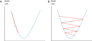
Cross entropy {as expressed in Eq. [10]} is set as a loss function for both training and validation. Adam optimization algorithm (41) is used to improve training. The Adam optimization will adjust learning rate automatically based on training performance to prevent slow coverage or oscillation of training (Figure 8) and also optimize weight adjustment for the BP during training. The initial learning rate is set to 1 × 10⁻⁵, while β1 and β2 of the Adam optimization are set to 0.1 and 0.001 respectively.
The network is also trained on Google Colab cloud server. The batch size is set to 32, so 32 images are used for each forward and back propagations. One training epoch is that all 14,820 images of training set were fed to the model once, so each epoch includes 14,820÷32≈464 batches of forward and back propagations. The network will be trained 300 iterations (approximately 7 hours) or until validation loss is not improved for 20 iterations with the powerful GPU of Google Colab. In our study, the training stopped at 71st iterations, which means that model was trained best at 51st epoch. The whole training process finally took approximately 2 hours. Figure 9 shows the model accuracy and loss of both training and validation sets. Only the best trained one will be saved and used for prediction.

Results
SVM data preprocessing
In order to extract more features for training in this work, 7 different filters selected manually are applied to the original image to generate 7 filtered images, each filtered image corresponding to a feature channel. These filters include Sobel filter (42), Gabor filter (43,44), Canny Edge filter (45), two Gaussian filters (46) with different parameters, Median filter, and Variance filter. This process is to extract some spatial information or relation of images. Thus, values of the filter parameters do not affect training results too much. Together with the original image, each sample now has 8 features (Figure 10).
SVM prediction and evaluation
One hundred and nine models are built for all 109 patients. The prediction results of one well-performed model is shown as follows.
For the patient A who has 6 images from dataset for test, the model achieved a training accuracy of 0.960. Figure 11 shows the prediction result with the ground truth.
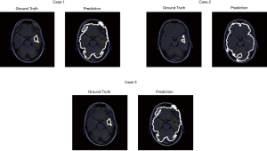
The contrast of MR images of some patients is not high, so some models perform not well. Patient B which has three images for test is one of patients whose MR image contrast is low (Figure 12). As shown in Figure 12, the contrast between glioma and normal tissue in MR images are low. It’s even difficult to identify glioma lesions manually.
Evaluations are based on model predictions of other testing images from the patient whose MR image is used to train the model. All models are evaluated after training.
For the model trained on patient A, the model achieved a reasonable prediction performance with an accuracy of 0.984, a precision of 0.689, a recall of 0.934, and an F1 score of 0.793. The confusion matrix of the model is presented in Table 2.

Full table
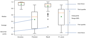
All 109 models are evaluated. Model performance in terms of Accuracy, Precision, Recall and F1 score are illustrated in boxplot (Figure 13), which is a method to graphically depict digital data sets by quartiles in descriptive statistics (47).
The four parameters used in model evaluations are also shown in Table 3. All models with F1 score smaller than 0.5 will be considered as models with poor performance. Sixty-seven models achieved F1 score greater than 0.5. Therefore, the SVM method used in this work is applicable to 67 of 109 patients.

Full table
CNN prediction and evaluation
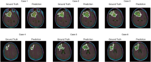
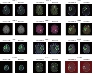
The test set consists of 276 MR images. The outputs are from Sigmoid function, so all of output value are between 0 and 1. All prediction pixels whose values are larger than 0.5 will be considered as a glioma tumor pixel. Figure 14 shows 12 randomly selected predictions and their corresponding ground truth.
CNN evaluation
All pixels of 276 images in test set are predicted by the model. The model achieves an accuracy of 0.998, a precision of 0.999, a recall of 0.999, and an F1 score of 0.999. It is nearly a perfect trained model. The confusion matrix is shown in Table 4.

Full table
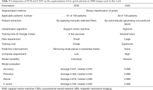
By comparing the training and performance of SVM and CNN method, similarities and differences between these two methods are concluded. Table 5 summarizes the comparison of SVM and CNN performances on the problem of segmenting MR images of this low-grade glioma of the brain.
Full table
Discussion
In the SVM method, only high contrast brain LGG MR images are applicable. The accuracy of the SVM model is relatively low in contrast to that achieved by using the CNN model, but its recall rate is relatively high, which indicates that the SVM model is sensitive enough to the target glioma pixels. Features are extracted by applying manually selected filters. The model learns from those features to generate its mathematic classification algorithm. In practice, different filters might be chosen for specific applications to gain the desired performance. However, in the SVM model developed for LGG MR image segmentation, manually selected types and parameters of the generic filters are not always able to fit the data well. This might negatively impact the performance of the SVM model. Additionally, the SVM model is a patient specific model and has to be trained for each individual patient.
A well-trained CNN usually predicts nearly perfectly if a significantly large data set is provided. The CNN model has multiple convolutional layers and consists of a large number of filters for feature extraction. The parameters or weights of the filters are automatically adjusted epoch by epoch according to the learning outcome in order to achieve an approximately perfect model. During the training process, image features are extracted layer by layer, and ultimately no complex algorithms are needed for classification. Unlike the SVM model, the trained CNN model is not patient specific and can segment brain LGG MR images in different patients.
Image quality of the dataset used for training SVM and CNN models might affect the performance of LGG MR image segmentation. Higher signal-to-noise ratio (SNR) and contrast-to-noise ratio (CNR) of the dataset should produce more accurate results although there is no linear relationship between SNR/CNR and F1-score in this study. Thus, using high field technique and advanced acquisition strategies for better SNR (48-54) and CNR (55-58) to generate training data should be advantageous for the LGG MR image segmentation.
The evaluation study indicates that the CNN model performs better than the SVM model on the brain low-grade glioma MR imaging segmentation problem. One of the reasons is that the CNN architecture contains a large number of parameters (usually millions) to deal with various complex problems. This fact requires high performance computers and long hours (usually dozens of hours) in model training. Compared to the CNN model, the SVM model requires much shorter time and has nearly no special requirements on the computing capability. The CNN model also requires a drastically large data set, which makes the training set expensive. In this work, the CNN model was trained by using thousands of MR images with manually created masks, while each SVM model requires only one MR image and mask pair as the training set. Therefore, the training set for SVM is much cheaper. Although in SVM, a specific model has to be built for each patient, the task is still manageable, given dramatically shortened computation time of only a few seconds.
Conclusions
In this study, two machine learning models, SVM and CNN, are developed for LGG MR image segmentation. The experimental results demonstrate that both SVM and CNN models are capable of segmenting LGG MR images reliably and accurately. Training of SVM model requires only one image per patient, which significantly shortens the computation time to a few seconds. The CNN model outperforms the SVM model in accuracy, precision, recall, and F1 score. But the training of the CNN model is slow, usually taking a few hours with high-performance computers, and also requires a significantly enlarged data set, which sometimes is not readily available in practice.
Acknowledgments
The authors would like to thank Ian Zhang for the technical discussions and scientific editing of the manuscript. The authors also thank Timothy O'Brien for the comments on the data analysis.
Funding: This work is supported in part by the grant from NIH (U01 EB023829) and SUNY Empire Innovation Professorship Award.
Footnote
Conflicts of Interest: All authors have completed the ICMJE uniform disclosure form (available at http://dx.doi.org/10.21037/qims-20-783). JX reports other from Sonioptix, LLC, outside the submitted work. XZ serves as an unpaid editorial board member of Quantitative Imaging in Medicine and Surgery, he reports grants from NIH and SUNY, during the conduct of the study. The other authors have no conflicts of interest to declare.
Open Access Statement: This is an Open Access article distributed in accordance with the Creative Commons Attribution-NonCommercial-NoDerivs 4.0 International License (CC BY-NC-ND 4.0), which permits the non-commercial replication and distribution of the article with the strict proviso that no changes or edits are made and the original work is properly cited (including links to both the formal publication through the relevant DOI and the license). See: https://creativecommons.org/licenses/by-nc-nd/4.0/.
References
- Goodenberger ML, Jenkins RB. Genetics of adult glioma. Cancer Genet 2012;205:613-21. [Crossref] [PubMed]
- Buda M, Saha A, Mazurowski MA. Association of genomic subtypes of lower-grade gliomas with shape features automatically extracted by a deep learning algorithm. Comput Biol Med 2019;109:218-25. [Crossref] [PubMed]
- Akkus Z, Galimzianova A, Hoogi A, Rubin DL, Erickson BJ. Deep Learning for Brain MRI Segmentation: State of the Art and Future Directions. J Digit Imaging 2017;30:449-59. [Crossref] [PubMed]
- Bousselham A, Bouattane O, Youssfi M, Raihani A. Towards Reinforced Brain Tumor Segmentation on MRI Images Based on Temperature Changes on Pathologic Area. Int J Biomed Imaging 2019;2019:1758948. [Crossref] [PubMed]
- Gordillo N, Montseny E, Sobrevilla P. State of the art survey on MRI brain tumor segmentation. Magn Reson Imaging 2013;31:1426-38. [Crossref] [PubMed]
- Wong KP. Medical Image Segmentation: Methods and Applications in Functional Imaging. In: Suri JS, Wilson DL, Laxminarayan S, editors. Handbook of Biomedical Image Analysis: Volume II: Segmentation Models Part B. Boston, MA: Springer US, 2005:111-82.
- Wang S, Su Z, Ying L, Peng X, Zhu S, Liang F, Feng D, Liang D. Accelerating magnetic resonance imaging via deep learning. 2016 IEEE 13th International Symposium on Biomedical Imaging (ISBI); 2016: IEEE.
- Schlemper J, Caballero J, Hajnal JV, Price AN, Rueckert D. A deep cascade of convolutional neural networks for dynamic MR image reconstruction. IEEE Trans Med Imaging 2018;37:491-503. [Crossref] [PubMed]
- Alpaydin E. Introduction to Machine Learning. Available online: https://www.udacity.com/course/intro-to-machine-learning--ud120
- Samuel AL. Some Studies in Machine Learning Using the Game of Checkers. IBM J Res Dev 1959;3:210-29. [Crossref]
- Lundervold AS, Lundervold A. An overview of deep learning in medical imaging focusing on MRI. Z Med Phys 2019;29:102-27. [Crossref] [PubMed]
- Mitchell T. The Discipline of Machine Learning. Available online: https://www.researchgate.net/publication/268201693_The_Discipline_of_Machine_Learning
- Liu J, Li M, Wang J, Wu F, Liu T, Pan Y. A Survey of MRI-Based Brain Tumor Segmentation Methods. Tsinghua Sci Technol 2014;19:578-95. [Crossref]
- Chapelle O, Schölkopf B, Zien A. Semi-Supervised Learning. Available online: http://www.acad.bg/ebook/ml/MITPress-%20SemiSupervised%20Learning.pdf
- Ruan S, Lebonvallet S, Merabet A, Constans J. Tumor segmentation from a multispectral MRI images by using support vector machine classification. Available online: https://ieeexplore.ieee.org/document/4193516
- Chen YY, Lin YH, Kung CC, Chung MH, Yen IH. Design and Implementation of Cloud Analytics-Assisted Smart Power Meters Considering Advanced Artificial Intelligence as Edge Analytics in Demand-Side Management for Smart Homes. Sensors (Basel, Switzerland) 2019;19:2047. [Crossref] [PubMed]
- Kayalıbay B, Jensen G, van der Smagt P. CNN-based Segmentation of Medical Imaging Data. Available online: https://arxiv.org/abs/1701.03056
- Cristianini N, Shawe-Taylor J, Shawe-Taylor DCSRHJ, Books24x7 I, Press CU. An Introduction to Support Vector Machines and Other Kernel-based Learning Methods. Cambridge University Press, 2000.
- Guo L, Liu X, Wu Y, Yan W, Shen X. Research on the segmentation of MRI image based on multi-classification support vector machine. Annu Int Conf IEEE Eng Med Biol Soc 2007;2007:6020-3. [PubMed]
- Nocedal J, Wright S. Numerical optimization. New York, NY: Springer Science & Business Media, 2006.
- Abbod MF, Catto JWF, Linkens DA, Hamdy FC. Application of Artificial Intelligence to the Management of Urological Cancer. J Urol 2007;178:1150-6. [Crossref] [PubMed]
- Dawson CW, Wilby R. An artificial neural network approach to rainfall-runoff modelling. Hydrol Sci J 1998;43:47-66. [Crossref]
- Goodfellow I, Bengio Y, Courville A. Deep Learning. Cambridge, Massachusetts: MIT Press, 2016.
- Cireşan DC, Giusti A, Gambardella LM, Schmidhuber J. Deep neural networks segment neuronal membranes in electron microscopy images. Lake Tahoe, Nevada: Curran Associates Inc., 2012;2:2843-51.
- Havaei M, Davy A, Warde-Farley D, et al. Brain tumor segmentation with Deep Neural Networks. Med Image Anal 2017;35:18-31. [Crossref] [PubMed]
- Kamnitsas K, Ledig C, Newcombe VFJ, et al. Efficient multi-scale 3D CNN with fully connected CRF for accurate brain lesion segmentation. Med Image Anal 2017;36:61-78. [Crossref] [PubMed]
- Milletari F, Navab N, Ahmadi SA. V-Net: Fully Convolutional Neural Networks for Volumetric Medical Image Segmentation. Available online: https://arxiv.org/abs/1606.04797
- Ronneberger O, Fischer P, Brox T. U-Net: Convolutional Networks for Biomedical Image Segmentation. Available online: https://arxiv.org/abs/1505.04597
- Çiçek Ö, Abdulkadir A, Lienkamp SS, Brox T, Ronneberger O. 3D U-Net: Learning Dense Volumetric Segmentation from Sparse Annotation. Available online: https://arxiv.org/abs/1606.06650
- Long J, Shelhamer E, Darrell T. Fully convolutional networks for semantic segmentation. Available online: https://arxiv.org/abs/1411.4038
- Powers DMW. Evaluation: from precision, recall and F-measure to ROC, informedness, markedness and correlation. Available online: https://www.researchgate.net/publication/276412348_Evaluation_From_precision_recall_and_F-measure_to_ROC_informedness_markedness_correlation
- Shobha G, Rangaswamy S. Chapter 8 - Machine Learning. In: Gudivada VN, Rao CR, editors. Handbook of Statistics. Amsterdam: Elsevier, 2018:197-228.
- Bharati MH, Liu JJ, MacGregor JF. Image texture analysis: methods and comparisons. Chemometr Intell Lab Syst 2004;72:57-71. [Crossref]
- Taylor L, Nitschke G. Improving deep learning using generic data augmentation. Available online: https://arxiv.org/abs/1708.06020
- Subramanian J, Simon R. Overfitting in prediction models - is it a problem only in high dimensions? Contemp Clin Trials 2013;36:636-41. [Crossref] [PubMed]
- Yaeger L, Lyon RF, Webb BJ. Effective training of a neural network character classifier for word recognition. Available online: https://papers.nips.cc/paper/1250-effective-training-of-a-neural-network-character-classifier-for-word-recognition
- Nair V, Hinton GE. Rectified linear units improve restricted boltzmann machines. Available online: https://www.cs.toronto.edu/~fritz/absps/reluICML.pdf
- Srivastava N, Hinton G, Krizhevsky A, Sutskever I, Salakhutdinov R. Dropout: a simple way to prevent neural networks from overfitting. J Mach Learn Res 2014;15:1929-58.
- He K, Zhang X, Ren S, Sun J. Delving Deep into Rectifiers: Surpassing Human-Level Performance on ImageNet Classification. Available online: https://arxiv.org/abs/1502.01852
- Berrar D. Cross-Validation. In: Ranganathan S, Gribskov M, Nakai K, et al. editors. Encyclopedia of Bioinformatics and Computational Biology. Oxford: Academic Press, 2019:542-5.
- Kingma DP, Ba J. Adam: A method for stochastic optimization. Available online: https://arxiv.org/abs/1412.6980
- Sobel I. An Isotropic 3x3 Image Gradient Operator. Available online: https://www.researchgate.net/publication/239398674_An_Isotropic_3x3_Image_Gradient_Operator
- Gabor D. Theory of communication. Part 1: The analysis of information. Available online: https://ieeexplore.ieee.org/document/5298517
- Daugman JG. Two-dimensional spectral analysis of cortical receptive field profiles. Vision Res 1980;20:847-56. [Crossref] [PubMed]
- Canny J. A computational approach to edge detection. IEEE Trans Pattern Anal Mach Intell 1986;8:679-98. [Crossref] [PubMed]
- Haddad RA, Akansu AN. A class of fast Gaussian binomial filters for speech and image processing. IEEE Trans Signal Process 1991;39:723-7. [Crossref]
- Wickham H, Stryjewski L. 40 years of boxplots. Available online: http://byrneslab.net/classes/biol607/readings/wickham_boxplots.pdf
- Zhang X, Ugurbil K, Chen W. Microstrip RF surface coil design for extremely high-field MRI and spectroscopy. Magn Reson Med 2001;46:443-50. [Crossref] [PubMed]
- Zhang X, Ugurbil K, Sainati R, Chen W. An inverted-microstrip resonator for human head proton MR imaging at 7 tesla. IEEE Trans Biomed Eng 2005;52:495-504. [Crossref] [PubMed]
- Zhang X, Ugurbil K, Chen W. A microstrip transmission line volume coil for human head MR imaging at 4T. J Magn Reson 2003;161:242-51. [Crossref] [PubMed]
- Zhang X. Sensitivity enhancement of traveling wave MRI using free local resonators: an experimental demonstration. Quant Imaging Med Surg 2017;7:170-6. [Crossref] [PubMed]
- Zhang X, Pang Y, Vigneron DB. SNR Enhancement by Free Local Resonators for Traveling Wave MRI. Available online: https://cds.ismrm.org/protected/14MProceedings/files/1357.pdf
- Yan X, Xue R, Zhang X. Closely-spaced double-row microstrip RF arrays for parallel MR imaging at ultrahigh fields. Appl Magn Reson 2015;46:1239-48. [Crossref] [PubMed]
- Wu B, Zhang X, Wang C, Li Y, Pang Y, Lu J, Xu D, Majumdar S, Nelson SJ, Vigneron DB. Flexible transceiver array for ultrahigh field human MR imaging. Magn Reson Med 2012;68:1332-8. [Crossref] [PubMed]
- Pang Y, Zhang X. Interpolated compressed sensing for 2D multiple slice fast MR imaging. PLoS One 2013;8:e56098. [Crossref] [PubMed]
- Pang Y, Zhang X. Interpolated Compressed Sensing MR Image Reconstruction using Neighboring Slice k-space Data. Available online: https://cds.ismrm.org/protected/12MProceedings/files/2275.pdf
- Pang Y, Jiang J, Zhang X. Ultrafast Fetal MR Imaging using Interpolated Compressed Sensing. Available online: https://cds.ismrm.org/protected/14MProceedings/files/2224.pdf
- Pang Y, Yu B, Zhang X. Enhancement of the low resolution image quality using randomly sampled data for multi-slice MR imaging. Quant Imaging Med Surg 2014;4:136-44. [PubMed]

