
A polarization-sensitive light field imager for multi-channel angular spectroscopy of light scattering in biological tissues
Introduction
Reliable detection of precancerous cells is an essential step to ensure timely treatments which can reduce the risk of malignant development of tumors. Biological cells undergo morphological changes during cancerous development. Histological biomarkers such as nuclear enlargement (1) and hyperchromasia (darker staining because of denser chromatin) (2,3) provide indicators for early diagnosis of precancerous cells. However, conventional histological examination requires biopsies which involve painful procedure and complicated sample preparation. It is known that light scattering characteristics in cells are sensitive to the size, distribution, and relative refractive index of subcellular scatters such as nuclei (4-6). Light scattering spectroscopy has been explored for vital study of subcellular organelles (7-10), cellular volume (11) and physiological condition of biological tissues (12). It promises a new methodology to complement histological examination for in vivo detection of precancerous and cancerous cells in optically accessible organs (13,14). Morphological and physiological abnormalities of cells or nuclei have been revealed by spectral and angular spectroscopy of scattered light. The spectral spectroscopy is employed to disclose wavelength (color) dependent differences; while the angular spectroscopy is used to detect angle-resolved changes in light scattering (9,15).
Angular distribution of light scattering has been known to be highly dependent on the orientation of tested specimens such as deformed elongated cells and well-packed fibers (16,17). The angular spectroscopy is typically implemented through a single-channel goniometric setup, which suffers from low spatial resolution or requires time-consuming scanning over extended area. Alternatively, angular resolution can be achieved by using a spatial filter at the Fourier plane that only allows scattered light with a specific scattering angle to pass through (18,19). However, this scheme requires physical manipulation of the spatial filter and it only samples one angle at a time which makes it time-consuming again for two-dimensional (2D) recording. Projecting the Fourier plane to the 2D camera could realize 2D recording of the scattering (11). However, this approach lacks the spatial resolution and the whole illuminated area could contribute to the scattering, which might overwhelm the useful signals. To address this issue, we developed a light field imager which employed a microlens array (MLA) at the image plane to realize 2D recording of the angular distribution of the light scattering while maintaining an acceptable spatial resolution. Polarization-sensitive recording capability was integrated to enable quantitative analysis of scattering signals at high sensitivity. Lobster leg nerves were employed to demonstrate polarization-sensitive light field differentiation of normal and unhealthy tissues. Experiments on the lobster leg nerves revealed 2D elliptical scattering patterns which were highly dependent on the orientation of the nerves, while as the nerves deteriorated, the elliptical scattering patterns gradually lost the ellipticity and became rotationally symmetric (i.e., circular). We anticipate that further development of the polarization-sensitive light field imager promises a method for in vivo screening of precancerous cells by rapid multi-channel angular spectroscopy at high resolution.
Materials and methods
Experimental setup
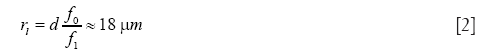
Figure 1A shows the optical diagram of polarization-sensitive light field imager. A near infrared (NIR) superluminescent diode (SLD-351, Superlum) was employed for illumination. The center wavelength was λ=830 nm and the band width was Δλ=60 nm. A 20× objective with 0.5 numerical aperture (NA) was used. The equivalent focal length of the objective was f0=9 mm in the air. Camera 1 was conjugate to the specimen for the position adjustment of the specimen. The MLA was also conjugate to the specimen. The back focal plane (i.e., Frourier plan) of the MLA was imaged to Camera 2. The lenslet of the MLA was rectangular. The length of each side was d=0.3 mm. The focal length of each lenslet was fm=3 mm. The red NIR light emission diode (LED) below the sample was used for light illumination to monitor the sample through Camera 1. It was turned off during light field imaging. According to the Rayleigh criteria, the angular resolution of the system was determined by the light wavelength, diameter of the lenslet of the MLA and optical magnification of the optical system:


where f1 was the focal length of the lens L1. The transverse resolution of the system was:
If we multiple Eq. [1] with Eq. [2], we obtain:

Eq. [3] indicates a tradeoff between spatial and angular resolutions for light field imaging.
A pair of crossed linear polarizers LP1 and LP2 was added to provide polarization-sensitive measurement. As shown in Figure 1B and Figure 2A, the lobster leg nerve bundle was placed at 45° with respect to the polarization direction of the incident light. The incident direction of the illumination light was along the z axis and perpendicular to long axis of the nerve fibers. The polarization plane (the gray plane in Figure 1B) of the incident light was parallel to the y-z plane.

Calculation of ellipticity
2D angular polarization-sensitive scattering patterns of the fresh nerves were elliptical (Figure 2B), while they became circular as the nerves physiologically deteriorated over time, after repeated electrical stimulations (Figure 2C). At intermediate states (Figure 3A), scattering patterns were less elliptical (Figure 3B-D). The ellipticity of an ellipse is defined as:

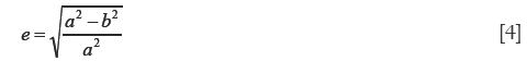
where a and b are major radius and minor radius of an ellipse, respectively. Intensity profiles of the scattering signals along the major axis (the x’ axis in Figure 3C,E) and the minor axis (the y’ axis in Figure 3C,E) were Gaussian distributed. The major radius a and the minor radius b of the ellipse were estimated by the full width at the half maximum of the Gaussian curve in the x’ axis and the y’ axis, respectively. If the ellipticity is 0, the scattering pattern is rotationally symmetric (i.e., circular), while the scattering pattern is a single line if the ellipticity is 1. It is an ellipse if the ellipticity is between 0 and 1.
Data fitting
To better understand the relationship between quantitative parameters (e.g., ellipticity and mean scattering intensity) and the peak-to-peak magnitude of the electrophysiological responses of the nerves M, curve fitting with least squares was applied. The fitting function employed in Figure 4A was:


where c1, c2 and c3 were coefficients estimated by data fitting. In contrast, the fitting function used in Figure 4B was a logistic function:
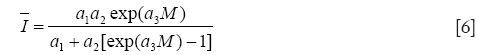
where a1, a2 and a3 were coefficients estimated by data fitting, and was the mean scattering intensity.
Specimen preparation
We used lobster leg nerves for experimental validation of the polarization-sensitive light field imaging system. The lobster leg nerves provide a simple anisotropic specimen for technical validation of 2D recording of the angular distribution. The 2D distribution profile underwent changes as the nerves deteriorated. We used the electrophysiological response of the nerves as the physiological biomarker of functional integrity of the nerves. All animal handling procedures were approved by the Institutional Animal Care and Use Committee of the University of Alabama at Birmingham. Details of the sample preparation have been reported in our previous publications (20). Briefly, the Furusawa pulling out method was applied to extract the nerves (21). The recording chamber was filled with the Ringer solution of lobster leg nerves. At the center of the chamber, a square cover glass was placed on the top of the recording chamber to reduce the effect of water fluctuation on the optical recording. A pair of silver electrodes was used to stimulate the nerves. Another pair of silver electrodes was used to record stimulus-evoked electrophysiological response of the nerves. Each stimulus pulse lasted for 0.1 ms. The current of the stimulus was 10 mA. Repeated stimulations were applied to accelerate physiological degeneration of the nerves. Scattering patterns of the nerves were recorded after every 20 stimulations.
Results
Figure 2 shows comparison of 2D angular polarization-sensitive scattering distribution between fresh and unhealthy lobster leg nerves. Figure 2A shows an image acquired by Camera 1 using the NIR LED illumination below the specimen. Figure 2A illustrates the orientation of the nerves. As shown in Figure 1B, the long axis of the nerves was parallel to the x-y plane and 45° with respect to the x axis (i.e., along the y’ axis in Figure 2A). Figure 2B shows elliptical scattering distribution patterns of the fresh nerves. The long axis of the ellipse was perpendicular to the orientation of the nerves. In contrast, as shown in Figure 2C, the deteriorated nerves showed more rotationally symmetric scattering patterns which were independent from the orientation of the nerves. Moreover, the scattering intensity of the deteriorated nerves was much weaker than that of the fresh nerves (intensity of the image Figure 2C was multiplied by a factor of 5 for a better view). We selected two areas, Area 1 (specified by yellow) and Area 2 (specified by green squares in Figure 2B) to better illustrate how the scattering distribution patterns were altered by the deterioration of the nerves.
Figure 3 shows that the ellipticity of the polarization-sensitive scattering patterns degraded when the nerves were physiologically deteriorated due to repeated electrical stimulations. Scattering patterns of two representative areas, Area 1 (Figure 3B) and Area 2 (Figure 3D), were illustrated. Figure 3A shows electrophysiological responses of the nerves with various magnitudes sequentially recorded at 20th, 160th, 220th and 480th stimulation, respectively. We used peak-to-peak magnitude of electrophysiological responses as a biomarker to represent the viability level of the nerves. Peak-to-peak magnitudes of four curves in Figure 3A were around 10, 4, 1.3 and 0.03 mV, respectively. Figure 3B,D shares a similar trend overall. First, the elliptical scattering patterns gradually became rotationally symmetric as the nerves got more degenerated. Second, the polarization-sensitive scattering intensity was decreased as the nerves lost the viability. The brightness of the second, third and fourth images in both Figure 3B,D was adjusted (multiplied by a factor of 1.5, 3 and 5, respectively) for a better view. Therefore, the intensity of images in both Figure 3B,D was decreased in sequence, although the presented images render similar brightness. As shown in Figure 3C,E, scattering intensity profiles along the x’ axis and the y’ axis at the region of interest 1 (ROI 1) and ROI 2 confirmed these two observations: the loss of the ellipticity and the decrease of scattering intensity due to the deterioration of the nerves.
Two quantitative parameters, the ellipticity as defined in Eq. [4] and the scattering intensity, were plotted as a function of the peak-to-peak magnitude of electrophysiological responses of the nerves. Figure 4A shows the values of the ellipticity of ROI 1 (specified by the white arrow in Figure 3B) and ROI 2 (specified by the white arrow in Figure 3D) as the nerves got deteriorated, while Figure 4B shows the mean of the scattering intensity of ROI 1 and ROI 2. To reliably compare the ellipticity and the mean of the scattering intensity between Area 1 and Area 2, we investigated all scattering subunits of Area 1 and Area 2 and plotted the data in Figure 4C,D. Shadow in Figure 4C,D indicates the standard deviation. In Figure 4C, the overall trend of the ellipticity at Area 1 and Area 2 was in common: the value of the ellipticity was high when the nerves were fresh and was decreased due to physiological deterioration of the nerves. However, distinct spatial variations existed. First, at any given point of the electrophysiological magnitude, Area 1 always had a smaller ellipticity value than Area 2. Second, the changing rate of Area 1 was bigger than that of Area 2, since the length of the green bar was longer than that of the black bar in Figure 4C. Figure 4D shows that both Area 1 and Area 2 had a decreased scattering intensity when the magnitudes of the electrophysiological responses were small because of the degeneration of the nerves. The length of the green bar was shorter than that of the black bar in Figure 4D, which implied that the scattering intensity of Area 1 decreased faster than that of Area 2 as the electrophysiological magnitude got smaller.
Discussion and conclusions
In summary, we developed a polarization-sensitive light field imager to conduct multi-channel [64] angular spectroscopy of light scattering with both spatial and angular resolutions. Light filed imaging of freshly isolated lobster leg nerves revealed elliptical scattering patterns (Figure 2B), which reflects highly orientation dependent light distributions. Values of the ellipticity and the scattering intensity were also location dependent. Area 1 always had a smaller ellipticity (Figure 4C) and a bigger scattering intensity (Figure 4D) comparing to Area 2. The spatial variations might attribute to localized difference of nerve fiber sizes and numbers (22). Comparative light field imaging and electrophysiological examination of freshly isolated and physiologically deteriorated lobster nerves was conducted to demonstrate the potential of light field identification of tissue dysfunctions. First, as the nerves got deteriorated, the elliptical scattering patterns became more and more rotationally symmetric (Figures 3,4A and C). Second, the mean scattering intensity was attenuated as the deterioration of the nerves got advanced. Moreover, this relationship was spatially various (Figure 4C,D), which demonstrated the advantage of the multi-channel imaging for reliable longitudinal (i.e., chronological) studies. Reflected polarization light signals might be produced by scattering (23) and birefringence (24). The disease or deterioration of the nerves might cause structural and morphological changes, e.g., disruption of well-organized cell membranes, alternation of refractive index, and cell swelling or shrinking, which could in turn lead to the change of optical properties of the nerves. The axial resolution of our current light field system is limited by the NA of the objective. To enhance the axial resolution, the optical coherence tomography technique can be integrated in future systems to gate the signal from individual depths (25,26). We anticipate that further development of polarization-sensitive light field imager promises a reliable strategy to screen precancerous cells in vivo at optically accessible organs to complement in vitro histological examination. The multi-channel angular spectroscopy is also providing an important tool to investigate biophysical mechanisms of transient polarization light changes in excitable nerve tissues (20,22).
Acknowledgements
This research is supported in part by NIH R21 EB012264, NIH R01 EY023522, NIH R01 EY024628, and NSF CBET-1055889.
Disclosure: The authors declare no conflict of interest.
References
- Yanofsky VR, Mercer SE, Phelps RG. Histopathological variants of cutaneous squamous cell carcinoma: a review. J Skin Cancer 2011;2011:210813.
- Bloom HJ, Richardson WW. Histological grading and prognosis in breast cancer; a study of 1409 cases of which 359 have been followed for 15 years. Br J Cancer 1957;11:359-77. [PubMed]
- Jeong JO, Han JW, Kim JM, Cho HJ, Park C, Lee N, Kim DW, Yoon YS. Malignant tumor formation after transplantation of short-term cultured bone marrow mesenchymal stem cells in experimental myocardial infarction and diabetic neuropathy. Circ Res 2011;108:1340-7. [PubMed]
- Kreysing M, Boyde L, Guck J, Chalut KJ. Physical insight into light scattering by photoreceptor cell nuclei. Opt Lett 2010;35:2639-41. [PubMed]
- Sloot PM, Figdor CG. Elastic light scattering from nucleated blood cells: rapid numerical analysis. Appl Opt 1986;25:3559. [PubMed]
- Mullaney PF, Dean PN. The small angle light scattering of biological cells. Theoretical considerations. Biophys J 1970;10:764-72. [PubMed]
- Mourant JR, Canpolat M, Brocker C, Esponda-Ramos O, Johnson TM, Matanock A, Stetter K, Freyer JP. Light scattering from cells: the contribution of the nucleus and the effects of proliferative status. J Biomed Opt 2000;5:131-7. [PubMed]
- Perelman LT, Backman V, Wallace M, Zonios G, Manoharan R, Nusrat A, Shields S, Seiler M, Lima C, Hamano T, Itzkan I, Van Dam J, Crawford JM, Feld MS. Observation of Periodic Fine Structure in Reflectance from Biological Tissue: A New Technique for Measuring Nuclear Size Distribution. Phys Rev Lett 1998;80:627-30.
- Mourant JR, Freyer JP, Hielscher AH, Eick AA, Shen D, Johnson TM. Mechanisms of light scattering from biological cells relevant to noninvasive optical-tissue diagnostics. Appl Opt 1998;37:3586-93. [PubMed]
- Wilson JD, Bigelow CE, Calkins DJ, Foster TH. Light scattering from intact cells reports oxidative-stress-induced mitochondrial swelling. Biophys J 2005;88:2929-38. [PubMed]
- Kinnunen M, Kauppila A, Karmenyan A, Myllylä R. Effect of the size and shape of a red blood cell on elastic light scattering properties at the single-cell level. Biomed Opt Express 2011;2:1803-14. [PubMed]
- Hofmann KP, Uhl R, Hoffmann W, Kreutz W. Measurements on fast light-induced light-scattering and -absorption changes in outer segments of vertebrate light sensitive rod cells. Biophys Struct Mech 1976;2:61-77. [PubMed]
- Mourant JR, Bigio IJ, Boyer J, Conn RL, Johnson T, Shimada T. Spectroscopic diagnosis of bladder cancer with elastic light scattering. Lasers Surg Med 1995;17:350-7. [PubMed]
- Mourant JR, Bocklage TJ, Powers TM, Greene HM, Dorin MH, Waxman AG, Zsemlye MM, Smith HO. Detection of cervical intraepithelial neoplasias and cancers in cervical tissue by in vivo light scattering. J Low Genit Tract Dis 2009;13:216-23. [PubMed]
- Drezek R, Dunn A, Richards-Kortum R. Light scattering from cells: finite-difference time-domain simulations and goniometric measurements. Appl Opt 1999;38:3651-61. [PubMed]
- Sacks MS, Smith DB, Hiester ED. A small angle light scattering device for planar connective tissue microstructural analysis. Ann Biomed Eng 1997;25:678-89. [PubMed]
- Arifler D, Macaulay C, Follen M, Guillaud M. Numerical investigation of two-dimensional light scattering patterns of cervical cell nuclei to map dysplastic changes at different epithelial depths. Biomed Opt Express 2014;5:485-98. [PubMed]
- Pyhtila JW, Wax A. Rapid, depth-resolved light scattering measurements using Fourier domain, angle-resolved low coherence interferometry. Opt Express 2004;12:6178-83. [PubMed]
- Gurjar RS, Backman V, Perelman LT, Georgakoudi I, Badizadegan K, Itzkan I, Dasari RR, Feld MS. Imaging human epithelial properties with polarized light-scattering spectroscopy. Nat Med 2001;7:1245-8. [PubMed]
- Lu RW, Zhang QX, Yao XC. Circular polarization intrinsic optical signal recording of stimulus-evoked neural activity. Opt Lett 2011;36:1866-8. [PubMed]
- Furusawa K. The depolarization of crustacean nerve by stimulation or oxygen want. J Physiol 1929;67:325-42. [PubMed]
- Schei JL, McCluskey MD, Foust AJ, Yao XC, Rector DM. Action potential propagation imaged with high temporal resolution near-infrared video microscopy and polarized light. Neuroimage 2008;40:1034-43. [PubMed]
- Yao XC, Foust A, Rector DM, Barrowes B, George JS. Cross-polarized reflected light measurement of fast optical responses associated with neural activation. Biophys J 2005;88:4170-7. [PubMed]
- Cohen LB, Keynes RD, Hille B. Light scattering and birefringence changes during nerve activity. Nature 1968;218:438-41. [PubMed]
- Lu RW, Curcio CA, Zhang Y, Zhang QX, Pittler SJ, Deretic D, Yao XC. Investigation of the hyper-reflective inner/outer segment band in optical coherence tomography of living frog retina. J Biomed Opt 2012;17:060504. [PubMed]
- Wang B, Lu R, Zhang Q, Yao X. Breaking diffraction limit of lateral resolution in optical coherence tomography. Quant Imaging Med Surg 2013;3:243-8. [PubMed]

