Fully automated lesion segmentation and visualization in automated whole breast ultrasound (ABUS) images
Introduction
In recent years, breast cancer has become one of the most common cancers. According to the American Cancer Society’s 2013 statistics, breast cancer is the second leading cause of death in women (1). The statistics of the Republic of China’s 103-year cancer registration report shows that there were 769 female breast cancer cases at that time, which was 593 more than the 176 cases 10 years ago, and the number increased by 90%. However, the initial symptoms of breast cancer are not easy to detect, and there will be obvious lumps and pains as the lesions spread. Therefore, early screening, tracking the efficacy of breast cancer treatments and chest reconstruction after breast cancer are very important.
Currently, breast cancer medical imaging is commonly performed using X-ray mammography, breast ultrasounds, and magnetic resonance imaging (MRI). The most common instruments used in breast cancer diagnosis are mammograms and breast ultrasound images. Among them, mammography is widely used for early screening. In general, 80–90% of breast cancer cases can be screened (2). However, since Asian women have higher breast density (3), X-ray photography is less sensitive and can yield false-positive results, which leads to overdiagnosis (4). In addition, X-ray photography compresses the breast during the examination, which causes pain for the subject. As a noninvasive testing method, the ultrasonic test has lower discomfort and the advantages of no radiation, immediacy, convenience and low cost. In addition, the illumination probe is highly flexible and can inspected over a wide range.
Conventional hand-held ultrasound (HHUS) images have been proved to be effective diagnostic tools and have been widely used in breast tumor diagnosis. However, two-dimensional information is missing. 2D probe breast tumor scanning ignores or misses small tumors. If only 2D scanned images are used to form judgments, important image features may be overlooked, such as whether a lesion exists or whether a lesion is benign or malignant. For example, common malignant tumors feature uneven bumps that cannot be clearly presented in 2D breast ultrasound images (5), making clinicians only able to make judgments with limited orientations and form uncertain diagnoses. Besides, a traditional sonogram produces a two-dimensional (2D) visualization of the breast and is highly operator dependent (6).
To overcome the lack of 2D breast ultrasound images, a supersonic imaging system manufacturer introduced a 3D ultrasound imaging system for breast examinations, the automated (whole) breast ultrasound system (ABUS), which is a probe. The entire breast is continuously scanned in a single direction and combined into an ABUS image. Since the automated whole breast ultrasound image covers the complete breast, it easily overcomes the possibility that the handheld breast ultrasound image misses a small tumor in the scan. It is one of the most breakthrough technologies in recent years (7). The ABUS is a safe, painless, nonradiative and noninvasive technology developed for whole breast imaging, and it uses 3D ultrasound technology that produces high-resolution images (8). It is known in other publications as the automated breast volume scanner (ABVS) and the automated whole breast scan (AWBS).
Why choose ABUS?
The mainstream first-line screening tool is mammography. However, a report published by the American College of Cancer Medicine in 2012 pointed out that mammography has a detection rate of less than 50% for dense breasts. Therefore, for Asian women, of which 70% of the population has dense breasts, mammography needs to be supplemented with breast ultrasound screening. Currently, breast ultrasounds are mostly manually operated with long operating times. Hence, it is difficult to produce standardized diagnostic images. Therefore, breast ultrasounds are not a first-line breast cancer screening tool. In the existing literature, the difference between the ABUS and HHUS has been studied. Lin et al. analyzed 81 cases (8). Both the ABUS and HHUS possess 100% sensitivity and high specificity (ABUS 95.0% and HHUS 85.0%). The diagnostic accuracy of the ABUS (97.1%) is higher than that of the HHUS (91.4%). In study (9), 15 cases of lesions under the nipple were examined by the ABUS and HHUS; however, in one of these cases, only the ABUS detected the lesion. Both studies indicated that the ABUS makes better judgments than the HHUS. Overall, ABUS could be successfully used in the visualization and characterisation of breast lesions (10).
The above literature shows many advantages of total breast ultrasounds. However, there are many diagnosis difficulties that need solving. The screening work needs to examine a considerable number of ABUS images, and each group of three-dimensional ABUS images involves hundreds of two-dimensional ultrasound images. In manual interpretation, it is easy to inadvertently miss smaller tumors. Second, even though the ABUS image contains sufficient structural information, the physician must still observe the three-dimensional structural information from various aspects, and there is still a lack of appropriate tools to evaluate important parameters, such as the distribution and shape of the lesion in space. Therefore, the detection and segmentation of lesions (implants or lesions) in ABUS images is important and necessary. The volume of breast lesions or tumors is an important preoperative parameter in order to predict the expected resection volume (11-13). The section volume in breast-conserving therapy is known to influence cosmetic outcomes (13-16). Precise measurement of the breast tumor volume is needed because of the preoperative prediction of the expected cosmetic outcome following breast-conserving therapy. To access these volumes, ABUS images were chosen since they have several advantages over other methods.
The lesions in this study are defined as lesions and implants placed in the breast. They may have weak boundaries or shadowing artifacts due to the attenuation effect of the ultrasonic signals traversing the path within the body. In addition, there are different kinds of breast lesions with different characteristics, such as hypoechoic lesions and hyperechoic lesions. These make it difficult to accurately segment lesions. To overcome the above difficulties, this study developed an automated lesion segmentation algorithm, including the automatic selection of a volume of interest (VOI). A series of 2D segmentation images are reconstructed into a 3D image to evaluate the segmentation accuracy, estimate the tumor’s volume, and visually represent the tumor for the physician.
Kozegar et al. (17) survey the method of different CADe systems for ABUS images and analysis the workflow and model of method. Ikedo et al. (18) proposed a fully automated method for segmenting breast tumors. In it, the Canny edge detector is used to detect edges. Morphological methods are used to classify the edges into approximate vertical and approximate horizontal edges. The region approximate vertical edge is marked as a candidate position of the tumor, and then the watershed marker position is used for segmentation to generate a candidate tumor region. Lo et al. (19) also applied the watershed method to extract potential anomalous regions in ABUS images. The watershed method collects blocks of similar intensity near the local minimum of the gray intensity, transforms them into a homogeneous region, and then divides the image into multiple blocks. The intensity and texture characteristics were analyzed to estimate the possible tumor areas. Kim (20) applied Otsu’s method and morphology to extract the lesions in ABUSs and then used feature extraction and a Support Vector Machines (SVM) classifier to screen whether each candidate region was a lesion. In this study, it was found that the candidate region boundary, the four adjacent average intensities and the standard deviation of the pixels best reflect the lesion characteristics. Chang et al. (21) developed an automated screening system. First, they preprocessed the image to improve its quality, and then they divided it into many regions according to the distribution of the grayscale values. Finally, they define seven features (darkness, uniformity, width-height ratio, area size, non-persistence, coronal area size, and region continuity) to determine whether it is a tumor area. Moon et al. (22) segmented tumors using a fast 3D mean shift method, which is used to remove speckled noise and separate tissue with similar properties.
Moon et al. (23) and Lo et al. (24) used fuzzy grouping to detect tumor candidate locations from ABUS images, but many nonlesion regions were identified as tumor candidate regions. To reduce the false positives, the study analyzed the grayscale intensity, morphology, position and size characteristics of the candidate regions, and linear regression models of these parameters were used to estimate the tumor likelihood of each pixel of a candidate tumor. In other words, the tumor boundaries could be simultaneously segmented.
Tan et al. (25) performed nipple and chest wall segmentation after the positions of the nipple and chest wall in ABUSs were marked by an expert. The method first extracts the characterization, speckle, contrast and depth of the voxel, and then it inputs these characteristics into the neural network to calculate the potential abnormalities likelihood map. A local maximum in the likelihood map and a set of candidate regions are formed in each image. These candidates are further processed in the second detection phase, including region segmentation, feature extraction, and final classification. Different classifiers were used for classification experiments, including neural networks, support vector machines, k-nearest neighbors, and linear discriminants, to detect lesion areas.
Tan et al. (26) proposed a dynamic programming method called helical scanning. The method combines the position of the tumor boundary with the centroid of the tumor in the depth direction. The algorithm can be summarized in five steps: (I) dynamic programming utilization to convert volume into 2D images, (II) edge detection, (III) addition of multiple scan directions to the spiral model, (IV) three-dimensional reconstruction, and (V) depth information utilization to improve the segmentation results. This study was applied to 78 cancerous tumor data samples and reached an average Dice coefficient of 0.73±0.14.
To sum up, these studies mainly relied on the texture extraction to find the candidate area of the tumor, and further to segment or detect the target (tumors).
The tumor segmentation algorithm can be roughly divided into four parts: (I) noise reduction, (II) candidate region segmentation, (III) feature extraction, and (IV) features analysis and the target segmentation. The first step reduces the speckles unique to the ultrasound image. The preprocessing is performed, and then the candidate region is calculated to serve as the main structure of the segmentation of the algorithm. The literature (19,23,24,27) has used the different methods to segment the candidate regions, extract multiple features to analyze and calculate the target region, and then segment the lesions. However, the third step and fourth step are time-consuming, the entire image must be analyzed and extract multiple features or creates a tessellation of the image domain in lots of small cells by the morphological watershed method (28). This study uses the deformable model to segment the target instead.
For deformable model, the level set method plays vital role in medical image processing and analysis (28). Moon et al. (27) also applied the level-set method to tumor segmentation and recombined 3D images to detect tumors in ABUS images. However, in Moon’s study, the VOI containing the tumor is selected by the user. Then, the level set method is applied for extraction of the tumor from the VOI. In which, the initial contour is necessary for the level-set method (29). In Moon’s study (27), the operator needs to select the seed points for the level set segmentation and the seed points were used for generation of the initial contour for segmentation. Therefore, it is more cumbersome to apply in practical operations.
In this study, we developed a fully automated segmentation algorithm for ABUS images. The VOIs are selected automatically, and then defining the seed point at the center of the VOIs, and generating the initial contour. For the segmentation problem, if the location of the seed point is defined, the region growth method is generally used for segmentation. Compared to the classical region growth method, the adaptive region growth method (based on local image attributes) is more robust to grayscale height changes (30-34). However, if the boundary has low contrast, it easily leaks and excessively grows; if the gray level of the target is not uniform, it results in the insufficient growth problem. This study corrects the intensity inhomogeneity region so that the region growth method can be applied in the homogenous region without generating a leakage (35). Then, the initial contour can be obtained automatically, and then applying it to the deformable model can accurately segment the two-dimensional image.
Methods
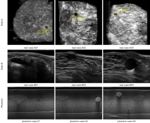
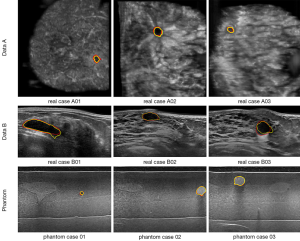
The Institutional Review Board approved the study, and all the experimental methods were carried out in accordance with the approved guidelines. In this study, the patients’ identities are removed from the images and data. The ABUS images are divided into two parts, which are the phantom cases (15 mass) and the real cases. To ensure the images’ robustness, the data of the real cases are collected from two machines so that the images from the different data sources look different. Dataset A is from Tan’s team (36), and it consists of 42 images, including 50 masses. These images are coronal views, and the image complexity is large. Dataset B consists of 16 images, including 20 masses. These images are circumferential orientation radial views, as shown as Figure 1. The third row of Figure 1 shows the phantom cases.
The architecture of the proposed algorithm in this study is shown in Figure 2. It can be divided into four parts: (I) volume of interest selection, (II) preprocessing, (III) segmentation, and (IV) visualization. First, a VOI is automatically selected using the three-dimensional level-set, and the rough boundary can be used as the parameter for the intensity inhomogeneity correction. Second, anisotropic diffusion is used to correct the speckled noise and intensity inhomogeneity to eliminate shadowing artifacts in the preprocessing step. Third, the adaptive distance regularization level set method (DRLSE) is used during the segmentation step to avoid the reinitialization of the segmentation curve in each evolution. The edge detection function of this model is modified by using the parameterized control curve evolution speed and is noise tolerant. Finally, the two-dimensional segmented images are reconstructed for visualization in the three-dimensional space.
The details of each step are detailed in the next section.
VOI selection
Generally, before lesion segmentation, the user first needs to manually define the VOI and select the target object in the middle of the VOI, which is beneficial to segmenting the boundary of the lesion.
Because of the many noises and artifacts in ABUS images, only rough or broken boundary information can be obtained using the three-dimensional level set method. This information can be used to automatically define the VOI range, and the rough foreground and background can be used as the parameters of the intensity inhomogeneity correction of the next step.
The level set is one algorithm that is used for image segmentation. The three-dimensional level set used in this study is based on the CV level set (29). Assuming that the VOI has already been defined, the energy function of the 3D level set is defined as follows.
The energy function of the C-V model is as follows:
|
| [1] |
where µ, λ1 and λ2 are fixed parameters and, generally, λ1, λ2=1; c1 and c2 are defined as the average gray level inside the variable curve C and the average gray level outside the variable curve C, respectively; and u0 is a given image. The first term of energy function is used to restrain the length of variable curve C. For 3D volumetric image data, u0(X):u0(x,y,z).
For the level set formulation, we replace the variable curve C with variable ϕ such that
|
| [2] |
The Heaviside function H and the one-dimensional Dirac measure δ0 are respectively defined as
|
| [3] |
Then, the energy function E(c1,c2,C) can be written as
|
| [4] |
By keeping c1 and c2 fixed and minimizing E respect to ϕ, we deduce the associated Euler-Lagrange equation for ϕ with an artificial time. To compute the equation for the unknown function ϕ, we consider slightly regularized versions of H and δ0, which are denoted by Hε and δε, where ε→0. The function can be given as follows:
|
| [5] |
We apply the abovementioned 3D level set model to 3D segmentation.
Pre-processing
For the speckled noise in ultrasonic images, anisotropic diffusion filtering is used. In addition, the intensity inhomogeneity correction (37) is used to reduce the postacoustic shadow or the lateral shadow around the lesion. This method is conducive to converging to a closed boundary when segmentation is performed using a deformation model.
Anisotropic diffusion
The Perona–Malik model is a nonlinear probability density function (PDF) (38), where the main partial differential equation of the model is Eq. [6], ∇I represents the gradient of the original image, the norm ‖∇I‖ is the edge detector, div represents the divergence operator, and c(x) represents the diffusion coefficient. There are two diffusion coefficient equations, which are represented by Eqs. [7,8], respectively.
|
| [6] |
|
| [7] |
|
| [8] |
In the anisotropic diffusion, the image gradient determines the degree of the image’s blurriness. Table 1 shows that the diffusion coefficient corresponds to the smoothness of the image. The anisotropic diffusion is very suitable for reducing the ultrasonic waves’ speckled noise since the ultrasonic speckled noise exhibits different intensities in different reflective materials. Therefore, using nonlinear filters reduces the speckled noise and preserves more boundary contrast.

Full table
Intensity inhomogeneity correction
Intensity inhomogeneity is a common issue in ABUS images. Shadowing artifacts usually reduce the image contrast and damage the true intensity.
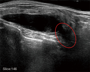
Therefore, intensity inhomogeneity greatly increases the difficulty of dividing the lesion contour. It is difficult to correctly segment the lesion contour. As shown in Figure 3, the object is easily segmented with leakage in the circled area. The abovementioned shadowing artifacts problem can be overcome by intensity inhomogeneity correction.
Presently, there are many studies (39-41) show that applying intensity inhomogeneity correction to an image can effectively improve the image’s quality, which achieves a better processing effect. There are many intensity inhomogeneity correction methods. For example, Sled et al. (42) regard intensity nonuniformity as a low-frequency signal and eliminate the offset field by means of a filter. However, this method has great risks and can result in the cancellation of important low frequency signals. Another common method is using polynomial or spline interpolation to calculate the best approximation surface (29).
It was assumed that the mean intensity inhomogeneity Pi of pixel i, ∀i, might be modeled as a polynomial surface, as defined in Eq. [9]. To estimate the polynomial surface, a least-squared fitting was employed to minimize the cost function as
|
| [9] |
where µΨ=µF if pixel i was in the foreground region and µΨ=µB if pixel i was in the background region. The rough boundaries are derived from the VOI selection step. Moreover, Pi=(xi,yi), where P(x,y) is a polynomial function of order n. In this study, n was set to 6.
Segmentation
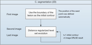
To segment specific lesions, this study develops an automated lesion segmentation algorithm. The algorithm’s flow chart is shown in Figure 4. The first image is defined by the VOI selection step. For example, there is a lesion in the range from the 85th to 220th images, where the 85th image is the first image. Using the long and short axes of the lesion on the first image, the seed point position can be automatically defined as well.
The boundary of the lesion is the initial contour of the subsequent segmentation process. The fine contour segmentation part uses the adaptive distance regularization level set method to minimize its functional energy formula so that the evolution contour curve is the edge of the target. Each image segmentation (t) result is used as the initial contour in the next image (t+1) to achieve a continuous segmentation effect.
Let y=f(x) denote a plane curve, and the implicit function form is y−f(x)=0. Then, the relationship with x and y can be written as shown in Eq. [10].
|
| [10] |
Given an initial closed curve C, the curve continuously evolves outward or inward along the normal direction at a certain speed. By introducing the time variable t, a set of curves C(t) is formed that changes with time to make it a higher dimensional space. The zero levels set of the surface function is {ϕ=0,t}, where ϕ(x,y,t) is a horizontal set function that varies with time. Li et al. proposed a DRLSE (43). The energy penalty term is introduced to automatically adjust the level set function to the symbol distance function, which avoids the problem of constantly initializing the zero level set function and constructing a distance normalization term. The external image drives the initial contour to the target contour position. The energy function can be defined as Eq. [11].
|
| [11] |
where Rp (ϕ) is the normalized term of the level set function ϕ’s normalization, µ>0 is a constant, and Eext (ϕ) is the external energy functional, which is the energy of the image region or curve.
The distance regularization level set evolution equation can be expressed as in Eq. [12].
|
| [12] |
where λ and α are weight parameters, and δε is a Dirac delta function.
The expression of g is given in Eq. [13], where Gσ is a Gaussian function with standard deviation σ, which reduces the noise; I represents an image; and * represents a convolution operation.
|
| [13] |
The above DRLSE model solves the problem that the traditional geometric contour mode needs to be continuously reinitialized. It has higher implementation efficiency and stable level set evolution. However, the DRLSE has the following disadvantages: the moving direction of the initial contour curve must be artificially set, and the evolution curve can only be set according to the setting. The direction shrinks or expands and evolves and cannot be autonomously changed according to the image features during the evolution process. If the expansion evolution motion is performed, the initial contour must be within the target boundary or outside the target boundary; if the contraction evolution motion is performed, the curve must contain the target outside the target. Once the initial contour curve intersects the target, it cannot be correctly segmented. Therefore, the DRLSE model fails to address the adaptive motion of the evolutionary curve and the sensitivity to the initial position.
Due to the above problems, this study analyzes Eq. [13]. The edge detection function that controls the evolution stop in the DRLSE model is sensitive to noise. If the noise is large, the evolution curve stays at the noise point and does not evolve. Therefore, the target object boundary cannot be reached. Further, the edge detection function acquires a large evolution speed at the weak boundary, resulting in inaccurate segmentation. For this reason, an adaptive parameter edge detection function shown in Eq. [14] is proposed.
|
| [14] |
where β>0 and γ>0 are constants. The evolution velocity parameter is used to adjust the evolution rate, and the noise sensitivity control parameter is used to control the sensitivity to noise.
Visualization of segmentation results
The whole breast ultrasonic instrument continuously scans in the circumferential direction. Therefore, it is necessary to convert the image into a coronal view in a cylindrical coordinate system; then, the isosurface rendering method is used to visualize the segmentation results.
The isosurface is the surface formed by the set of points with the same value in space. In the three-dimensional space, if each point F(x, y, z) having an equivalent value constitutes a curved surface, any point on the surface satisfies Eq. [15].
|
| [15] |
However, calculating F(x, y, z) is a complicated process. This study uses the high resolution 3D surface construction algorithm of marching cubes proposed by Lorenson and Cline in 1987 (44). The algorithm is widely used in 3D data display.
Results
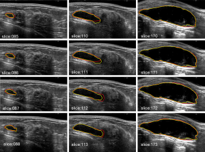
The ground truth is delineated by two radiologists with more than 10 years of experience in breast sonography. To demonstrate the effect of the proposed algorithm for ABUS images, Figure 5 shows the segmentation result of the proposed algorithm. The yellow line is the boundary derived by the proposed algorithm, and the red line is the corresponding mean manually delineated boundary. The sequence image results are presented in Figure 6. It can be seen that there is not much difference between the result derived by the proposed algorithm and the ground truth.
Visualization of segmentation results
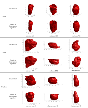
The 2D segmentation images are reconstructed to three-dimensional image by a cylindrical coordinate transformation, and the isosurface rendering is applied to it, as shown as Figure 7.
To quantify the segmentation results, three performance assessments are carried out to evaluate the effectiveness of the proposed algorithm in this study. The first assessment is the similarity measurement (45). The second assessment is the volume estimation of phantom cases.
The first assessment
There are four indicators of the similarity (43): the similarity index (SI), which is also called the Dice similarity index (Dice); the overlap fraction (OF); the overlap value (OV); and the extra fraction (EF), which is defined by Eqs. [16-19]. REF is the ground truth, and SEG is the boundary derived by the proposed algorithm.
|
| [16] |
|
| [17] |
|
| [18] |
|
| [19] |
The similarity measures of the 2D and 3D image segmentation results are calculated, as shown in Table 2 and Table 3, respectively.

Full table

Full table
In the 2D validation, the area Dice similarity coefficients of the real cases A, real cases B and phantoms are 0.84±0.02, 0.86±0.03 and 0.92±0.02, respectively. The OF and OV of the real cases A are 0.84±0.06 and 0.78±0.04, real case B are 0.91±0.04 and 0.82±0.05, respectively. The OF and OV of the phantoms are 0.95±0.02 and 0.92±0.03, respectively. In the 3D validation, the volume Dice similarity coefficients of the real cases A, real cases B and phantoms are 0.85±0.02, 0.89±0.04 and 0.94±0.02, respectively. The OF and OV of the real cases A are 0.82±0.06 and 0.79±0.04, real cases B are 0.92±0.04 and 0.85±0.07, respectively. The OF and OV of the phantoms are 0.95±0.01 and 0.93±0.04, respectively.
The second assessment
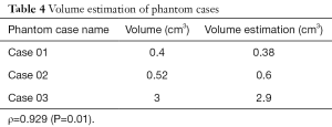
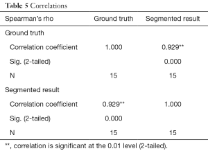
In this study, the volume is calculated from the segmented results, as shown in Table 4, and the accuracy of the segmentation results can be further verified. The Spearman’s correlation coefficient between the segmented volumes and the corresponding ground truth volumes is ρ=0.929 (P=0.01), as Table 5. Because there is only a gold standard answer in the phantom case, this study only evaluated the volume of the phantom case.
Full table
Full table
Discussion
The Chan-Vese level set method would not able to detect the weak edges of the lesion boundaries degraded by the intensity inhomogeneity. For all cases, from the three kinds of data sources, the zero level sets leak out of the lesions via the weak edge portions of the lesion boundaries, as shown in Figure 8. Figure 8 shows the lesion boundaries derived by the proposed algorithm and the Chan-Vese level set method with the same initial contours, respectively.
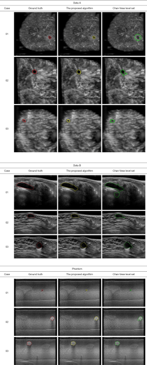
Table 6 shows the SI, i.e., the Dice index, between the boundaries derived by the proposed algorithm, the Chan-Vese level set method and the corresponding mean manually delineated boundaries. The Dice of the proposed algorithm in real cases A, real cases B and phantoms are 0.84±0.02, 0.86±0.03 and 0.92±0.02, respectively. The Dice of Chan-Vese level set in real cases A, real cases B and phantoms are 0.65±0.23, 0.69±0.14 and 0.76±0.14, respectively. A paired t-test for the Dice performance yields a P value of less than 0.01. The segmentation results of the proposed algorithm are better than those of the Chan-Vese level set method. It is evident that the weak edge problem that resulted from intensity inhomogeneity in ABUS images may be alleviated by the proposed algorithm.

Full table
Conclusions
The advancement of automated whole breast ultrasound technology has resulted in a large demand for the quantitative evaluation of lesions in three-dimensional ultrasonic images. However, ultrasonic images have multiple types of noise, such as speckled noise and shadowing artifacts, which make lesion segmentation quite difficult. In this study, the VOI can be automatically defined. Anisotropic diffusion was used to eliminate the speckled noise, and the intensity inhomogeneity correction was used to eliminate the shadowing artifacts at the edge of the lesion. The segmentation part adopts the adaptive DRLSE level set model, and it uses a parametric regulation model to change the sensitivity of the curve to noise, adjust the curve evolution speed of strong or weak boundaries, and increase the flexibility of the curve evolution. It can more accurately segment lesion regions. This study has a high degree of credibility for lesion segmentation. It can be combined with deep learning to identify benign and malignant lesions in the future and could greatly improve the diagnostic value of breast ultrasounds.
Acknowledgments
Funding: The authors acknowledge partial financial support from the Ministry of Science and Technology of the Republic of China (ROC), Taiwan (MOST 107-2221-E-239-010-MY3).
Footnote
Conflicts of Interest: The authors have no conflicts of interest to declare.
Ethical Statement: The Institutional Review Board approved the study, and all the experimental methods were carried out in accordance with the approved guidelines. In this study, the patients’ identities are removed from the images and data.
Open Access Statement: This is an Open Access article distributed in accordance with the Creative Commons Attribution-NonCommercial-NoDerivs 4.0 International License (CC BY-NC-ND 4.0), which permits the non-commercial replication and distribution of the article with the strict proviso that no changes or edits are made and the original work is properly cited (including links to both the formal publication through the relevant DOI and the license). See: https://creativecommons.org/licenses/by-nc-nd/4.0/.
References
- Siegel RL, Miller KD, Fedewa SA, Ahnen DJ, Meester RG, Barzi A, Jemal A. Colorectal cancer statistics, 2017. CA Cancer J Clin 2017;67:177-93. [Crossref] [PubMed]
- American Cancer Society. Breast cancer facts & figures. American Cancer Society 2007.
- del Carmen MG, Halpern EF, Kopans DB, Moy B, Moore RH, Goss PE, Hughes KS. Mammographic breast density and race. AJR Am J Roentgenol 2007;188:1147-50. [Crossref] [PubMed]
- Byrne C, Schairer C, Wolfe J, Parekh N, Salane M, Brinton LA, Haile R. Mammographic features and breast cancer risk: effects with time, age, and menopause status. J Natl Cancer Inst 1995;87:1622-9. [Crossref] [PubMed]
- Watermann DO, Földi M, Hanjalic‐Beck A, Hasenburg A, Lüghausen A, Prömpeler H, Stickeler E. Three-dimensional ultrasound for the assessment of breast lesions. Ultrasound Obstet Gynecol 2005;25:592-8. [Crossref] [PubMed]
- Agarwal R, Diaz O, Lladó X, Gubern-Mérida A, Vilanova JC, Martí R. Lesion Segmentation in Automated 3D Breast Ultrasound: Volumetric Analysis. Ultrason Imaging 2018;40:97-112. [Crossref] [PubMed]
- Wenkel E, Heckmann M, Heinrich M, Schwab SA, Uder M, Schulz-Wendtland R, Janka R. Automated Breast Ultrasound: Lesion Detection and BI-RADS™ Classification–a Pilot Study. In RöFo-Fortschritte auf dem Gebiet der Röntgenstrahlen und der bildgebenden Verfahren 2008;80:804-8.
- Lin X, Wang J, Han F, Fu J, Li A. Analysis of eighty-one cases with breast lesions using automated breast volume scanner and comparison with handheld ultrasound. Eur J Radiol 2012;81:873-8. [Crossref] [PubMed]
- Isobe S, Tozaki M, Yamaguchi M, Ogawa Y, Homma K, Satomi R, Fukuma E. Detectability of breast lesions under the nipple using an automated breast volume scanner: comparison with handheld ultrasonography. Jpn J Radiol 2011;29:361-5. [Crossref] [PubMed]
- Vourtsis A, Kachulis A. The performance of 3D ABUS versus HHUS in the visualisation and BI-RADS characterisation of breast lesions in a large cohort of 1,886 women. Eur Radiol 2018;28:592-601. [Crossref] [PubMed]
- Clauser P, Londero V, Como G, Girometti R, Bazzocchi M, Zuiani C. Comparison between different imaging techniques in the evaluation of malignant breast lesions: Can 3D ultrasound be useful? Radiol Med 2014;119:240-8. [Crossref] [PubMed]
- Krekel NMA, Zonderhuis BM, Stockmann HBAC, Schreurs WH, Van Der Veen H, de Klerk EDL, Meijer S, Van Den Tol MP. A comparison of three methods for nonpalpable breast cancer excision. Eur J Surg Oncol 2011;37:109-15. [Crossref] [PubMed]
- Taylor ME, Perez CA, Halverson KJ, Kuske RR, Philpott GW, Garcia DM, Morti-mer JE, Myerson RJ, Radford D, Rush C. Factors influencing cosmetic results after conservation therapy for breast cancer. Int J Radiat Oncol Biol Phys 1995;31:753-64. [Crossref] [PubMed]
- Vrieling C, Collette L, Fourquet A, Hoogenraad WJ, Horiot JC, Jager JJ, Pierart M, Poortmans PM, Struikmans H, Maat B, Van Limbergen E, Bartelink H. The influence of patient, tumor and treatment factors on the cosmetic results after breast-conserving therapy in the EORTC ‘boost vs. no boost’ trial. Radiother Oncol 2000;55:219-32. [Crossref] [PubMed]
- Cochrane RA, Valasiadou P, Wilson ARM, Al-Ghazal SK, Macmillan RD. Cosmesis and satisfaction after breast-conserving surgery correlates with the percentage of breast volume excised. Br J Surg 2003;90:1505-9. [Crossref] [PubMed]
- Chan SW, Chueng Polly SY, Lam SH. Cosmetic outcome and percentage of breast volume excision in oncoplastic breast conserving surgery. World J Surg 2010;34:1447-52. [Crossref] [PubMed]
- Kozegar E, Soryani M, Behnam H, Salamati M, Tan T. Computer aided detection in automated 3-D breast ultrasound images: a survey. Artif Intell Rev 2019.1-23.
- Ikedo Y, Fukuoka D, Hara T, Fujita H, Takada E, Endo T, Morita T. Development of a fully automatic scheme for detection of masses in whole breast ultrasound images. Med Phys 2007;34:4378-88. [Crossref] [PubMed]
- Lo CM, Chen RT, Chang YC, Yang YW, Hung MJ, Huang CS, Chang RF. Multi-dimensional tumor detection in automated whole breast ultrasound using topographic watershed. IEEE Trans Med Imaging 2014;33:1503-11. [Crossref] [PubMed]
- Kim JH, Cha JH, Kim N, Chang Y, Ko MS, Choi YW, Kim HH. Computer-aided detection system for masses in automated whole breast ultrasonography: development and evaluation of the effectiveness. Ultrasonography 2014;33:105. [Crossref] [PubMed]
- Chang RF, Chang‐Chien KC, Takada E, Huang CS, Chou YH, Kuo CM, Chen JH. Rapid image stitching and computer‐aided detection for multipass automated breast ultrasound. Med Phys 2010;37:2063-73. [Crossref] [PubMed]
- Moon WK, Lo CM, Chen RT, Shen YW, Chang JM, Huang CS, Chang RF. Tumor detection in automated breast ultrasound images using quantitative tissue clustering. Med Phys 2014;41:042901. [Crossref] [PubMed]
- Moon WK, Shen YW, Bae MS, Huang CS, Chen JH, Chang RF. Computer-aided tumor detection based on multi-scale blob detection algorithm in automated breast ultrasound images. IEEE Trans Med Imaging 2013;32:1191-200. [Crossref] [PubMed]
- Lo C, Shen YW, Huang CS, Chang RF. Computer-aided multiview tumor detection for automated whole breast ultrasound. Ultrasonic imaging 2014;36:3-17. [Crossref] [PubMed]
- Tan T, Platel B, Mus R, Tabar L, Mann RM, Karssemeijer N. Computer-aided detection of cancer in automated 3-D breast ultrasound. IEEE Trans Med Imaging 2013;32:1698-1706. [Crossref] [PubMed]
- Tan T, Gubern‐Mérida A, Borelli C, Manniesing R, van Zelst J, Wang L, Karssemeijer N. Segmentation of malignant lesions in 3D breast ultrasound using a depth‐dependent model. Med Phys 2016;43:4074-84. [Crossref] [PubMed]
- Moon WK, Shen YW, Huang CS, Chiang LR, Chang RF. Computer-aided diagnosis for the classification of breast masses in automated whole breast ultrasound images. Ultrasound Med Biol 2011;37:539-48. [Crossref] [PubMed]
- Moazzam MG, Chakraborty A, Nasrin S, Selim M. Medical Image Segmentation Based on Level Set Method. IOSR Journal of Computer Engineering (IOSR-JCE) 2013;10:35-41.
- Chan TF, Vese LA. Active contours without edges. IEEE Trans Image Process 2001;10:266-77. [Crossref] [PubMed]
- Yau HT, Lin YK, Tsou LS, Lee CY. An adaptive region growing method to segment inferior alveolar nerve canal from 3D medical images for dental implant surgery. Computer-Aided Design and Applications 2008;5:743-52. [Crossref]
- Roura E, Oliver A, Cabezas M, Vilanova JC, Rovira À, Ramió-Torrentà L, Lladó X. MARGA: multispectral adaptive region growing algorithm for brain extraction on axial MRI. Comput Methods Programs Biomed 2014;113:655-73. [Crossref] [PubMed]
- Li H, Thorstad WL, Biehl KJ, Laforest R, Su Y, Shoghi KI, Lu W. A novel PET tumor delineation method based on adaptive region‐growing and dual‐front active contours. Med Phys 2008;35:3711-21. [Crossref] [PubMed]
- Cao Y, Hao X, Zhu X, Xia S. An adaptive region growing algorithm for breast masses in mammograms. Frontiers of Electrical and Electronic Engineering in China 2010;5:128-36. [Crossref]
- Grenier T, Revol-Muller C, Costes N, Janier M, Gimenez G. 3D robust adaptive region growing for segmenting [18F] fluoride ion PET images. In Nuclear Science Symposium Conference Record, IEEE 2006;5:2644-8.
- Cary TW, Conant EF, Arger PH, Sehgal CM. Diffuse boundary extraction of breast masses on ultrasound by leak plugging. Med Phys 2005;32:3318-3328. [Crossref] [PubMed]
- Kozegar E, Soryani M, Behnam H, Salamati M, Tan T. Mass segmentation in automated 3-D breast ultrasound using adaptive region growing and supervised edge-based deformable model. IEEE Trans Med Imaging 2018;37:918-928. [Crossref] [PubMed]
- Lee CY, Chou YH, Huang CS, Chang YC, Tiu CM, Chen CM. Intensity inhomogeneity correction for the breast sonogram: Constrained fuzzy cell‐based bipartitioning and polynomial surface modeling. Med Phys 2010;37:5645-54. [Crossref] [PubMed]
- Perona P, Malik J. Scale-space and edge detection using anisotropic diffusion. IEEE Transactions on pattern analysis and machine intelligence 1990;12:629-39. [Crossref]
- Dawant BM, Zijdenbos AP, Margolin RA. Correction of intensity variations in MR images for computer-aided tissue classification. IEEE Trans Med Imaging 1993;12:770-81. [Crossref] [PubMed]
- Vemuri P, Kholmovski EG, Parker DL, Chapman BE. Coil sensitivity estimation for optimal SNR reconstruction and intensity inhomogeneity correction in phased array MR imaging. In Biennial international conference on information processing in medical imaging 2005;603-14.
- Gerig G, Prastawa M, Lin W, Gilmore J. Assessing early brain development in neonates by segmentation of high-resolution 3T MRI. In International Conference on Medical Image Computing and Computer-Assisted Intervention 2003;979-80.
- Sled JG, Zijdenbos AP, Evans AC. A nonparametric method for automatic correction of intensity nonuniformity in MRI data. IEEE Trans Med Imaging 1998;17:87-97. [Crossref] [PubMed]
- Li C, Xu C, Gui C, Fox MD. Distance regularized level set evolution and its application to image segmentation. IEEE Trans Image Process 2010;19:3243. [Crossref] [PubMed]
- Lorensen WE, Cline HE. Marching cubes: A high resolution 3D surface construction algorithm. ACM siggraph computer graphics 1987;21:163-9. [Crossref]
- Anbeek P, Vincken KL, Van Osch MJ, Bisschops RH, Van Der Grond J. Probabilistic segmentation of white matter lesions in MR imaging. NeuroImage 2004;21:1037-44. [Crossref] [PubMed]


