Generalized parameter estimation in multi-echo gradient-echo-based chemical species separation

Introduction

Multi-echo gradient echo imaging is a powerful imaging method in the range of quantitative MRI paradigms. Techniques like chemical shift encoding-based water-fat separation (1), fatty acid composition mapping (2), myelin water imaging (3), chemical shift encoding-based separation of metabolites (4), and quantitative susceptibility mapping (QSM) (5) have been based on multi-echo gradient-echo imaging to quantify spatially-resolved maps of the proton density fat fraction, the fat unsaturation, the myelin water fraction, the metabolite concentrations and the mean tissue magnetic susceptibility, respectively.

The analysis of multi-echo gradient-echo imaging measurements is typically based on the complex MR data. Specifically, the excitation pulse of most multi-echo gradient-echo sequences has a finite bandwidth and thus not only protons at the center frequency are excited but also other chemical species, molecules with different chemical shifts, contribute to the MR signal formation. By sampling the MR signal at multiple echo times after the excitation pulse in a multi-echo gradient-echo imaging experiment, the presence of the different chemical species is encoded in the total MR signal. After the reconstruction of the single echo images, an assumed signal model is typically fit to the complex signal evolution measured at each image voxel. There is a plethora of different signal models that has been used in the literature (2,6-10). It is typically necessary to select the sampled echo times based on the noise properties of the assumed signal model (11) and to derive a parameter estimation scheme, often involving analytical computation of the derivatives with respect to the parameters of interest (1). Most existing works provide experimental design and parameter estimation strategies tailored to the details of the assumed signal model. Therefore, comparison of signal models requires reproduction of the methods from different sources, like previously attempted for the chemical shift encoding-based water-fat separation within the ISMRM fat-water toolbox (12).

The purpose of the present work is to develop a generalized formulation of multi-echo gradient-echo-based chemical species separation for all MR signal models described by a weighted sum of complex exponentials with phases linear in echo time and to provide parameter estimation for such signal models using an open source software framework based on the conventions of the ISMRM fat-water toolbox.

Methods

Generally, the complex MR signal in one voxel $s_n=s\left(t_n\right)$ , sampled at echo times $t_n,n=1,\mathrm{...},N$, behaves according to

where the contribution to the signal from every chemical species m=1,..,M is characterized by its magnitude ϱ_m, phase after the RF-excitation (at t=0) ϕ_m, resonance frequency ω_m and transverse relaxation rate R_m.

Since estimating the whole set of model parameters {ϱ_m,ϕ_m,ω_m,R_m}, m=1,..,M would require an impractical amount of observations S_n, it is necessary to reduce the number of parameters on the right hand side of Eq. [1]. Model parameters can be fixed by a priori values or constraints based on physically meaningful assumptions. Relations between different parameters can be incorporated by inserting indicator functions in the partial derivatives of Eq. [1]:

where the indicator functions

can be scaled with constant factors c to fix certain relational parameter assumptions. Notationally we distinguish free model parameters to be estimated with a hat and refer to their whole set as $\beta \text{=}\left\{\widehat{\varrho },\widehat{\varphi },\widehat{\omega },\widehat{R}\right\}$. An example for a possible model-specific parameter relation is given by the indicator function

where compared to Eq. [3] the following substitutions were made: $a={\widehat{R}}_1,b=R_m,c=1$. The indicator function Eq. [4] states that in such a signal model, there is only one free relaxation variable ${\widehat{R}}_1$ to be estimated and all relaxation rates of the other chemical species R_m, m=2,.., M behave according to the same partial derivative Eq. [2d]. As shown in the next section, the indicator functions can be combined to so-called constraint matrices that capture all parameter relations of one parameter type (ρ,ϕ,ω,R) across all chemical species m=1,.., M.

Matrix formulation

Starting from the general signal Eq. [1], we can write the voxel signal model in a multi-observation matrix formulation as

where we defined

with omitted matrix entries being zero. In the matrix notation Eq. [5], the parameter relations described by the indicator functions Eq. [3] can be defined as constraint matrices C _x, x∊{ϱ,ϕ,ω,r}, in the same way as the Kronecka symbol δ_ij corresponds to the entries of an identity matrix. For the example of indicator functions Eq. [4]—for signal models in which all relaxation rates are constrained by $R_{m>1}={\widehat{R}}_1$ —the corresponding constraint matrix is given by

In general, the constraint matrices corresponding to the indicator functions Eq. [3] are square with the same row number as the number M of present chemical species. The upper triangular part in each constraint matrix holds only zeros. Nonzero elements on the diagonal represent the parameters of interest that are solved for in the parameter estimation (the first entry of the example C _R Eq. [7] corresponding to the free variable ${\widehat{R}}_1$). Non-zero elements on the lower triangular part of the matrices describe constrained parameters based on the specific relations of the chosen model {corresponding to R_m>2 in Eq. [4]}. As columns of all zeros in the constraint matrices do not hold any information about parameter relations, they are removed, which reduces the matrix sizes and avoids rank-deficiencies. Consequently, nonzero elements of corresponding parameter of interest might not be on the diagonal of the resulting rectangular matrices any more, but the number of model unknowns is represented by the column number of all constraint matrices after the removal of the zero-columns. In the above Eq. [7], the constraint matrix is consequently reduced to rectangular size M×1,

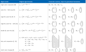
Further examples for sets of constraint matrices for common signal models in literature are given in the Results section. Thereby, we show the full square constraint matrices visualizing the full indicator functions of each parameter constraint before the removal of zero-columns. The constraint matrices with zero-columns removed are summarized in Figure 1.

Figure 1 Common complex-based MR signal models and their representations as sets of constraint matrices in the proposed generalized formulation for chemical species separation (2,3,7,10,11,13-16).

With all indicator functions in Eq. [3] combined to constraint matrices, the Jacobian for signal models of the form Eq. [1] can be written as

where $T=\text{diag}\left(t_1,\mathrm{...},t_N\right)$ and $D=\text{diag}\left(P\widehat{\varrho }\right)$. With the generalized Jacobian [9] one can formulate parameter estimation as well as an optimal echo time selection algorithm for all models of the class Eq. [1]. As shown in the next sections, the model-specific constraint matrices then become input parameters for the algorithms.

Parameter estimation

The generalized formulation of the Jacobian in Eq. [9] allows to develop a parameter estimation algorithm that is independent of an a priori choice of the signal model: The concrete specification of the constraint matrices can be treated as final input to the algorithm, which is written down in terms of unspecified constraint matrices. With the multi-observation formulation Eq. [6], the parameter estimation problem can be cast as the following minimization of the norm of the residual vector e ,

The above optimization problem can be iteratively solved via alternating Gauss-Newton updates of the linear ${\beta }_{\text{lin}}=\widehat{\varrho }$ ) and nonlinear parameters (${\beta }_{nonlin}\text{=}\left\{\widehat{\varphi },\widehat{\omega },\widehat{R}\right\}$ ) in Eq. [1] in a variable projection method (VARPRO) (17).

where B⁺ refers to the Moore-Penrose pseudo inverse, B⁺ =(A^†A )⁻¹P^†A^† , A^† is the Hermitian conjugate of A , and similarly for J⁺ . Note that the pseudo-code, hereafter Algorithm 1, largely resembles previously developed algorithms in water-fat imaging like the “Iterative Decomposition of water and fat with Echo Asymmetry and Least-squares estimation” (IDEAL) (18) or the VARPRO variant (19), but is not specific to the voxel signal model thanks to the use of the generalized Jacobian J .

The initialization ${\beta }_{\text{nonlin}}^{(0)}$ needs to be close enough to the global minimum of the residual norm to ensure convergence to the true parameter values, which is typically achieved by an initialization of the nonlinear parameters $\widehat{\omega }$ by global methods incorporating voxel neighborhood information (20-23). The iteration is stopped after N_max steps.

Noise performance analysis

Based on the noise properties of the assumed signal model—fixed by the choice of constraint matrices—the MR experiments can be optimally designed e.g., in terms of the selection of echo times. The typically employed Cramér-Rao lower bound (CRLB) on the minimal noise variance is based on the Fisher Information Matrix (FIM) defined as the expectation value ($\mathbb{E}[\dots ]$ ) of the second derivative of the log-likelihood $\text{ln}\mathcal{L}$,

where the likelihood

and the definitions from Eq. [6] apply. In the case of additive white Gaussian noise with variance σ², it can be shown (24) that the FIM is given by

with the Jacobian J from Eq. [9]. Therefore, the FIM can be generally written as

The Cramér-Rao lower bounds on the parameter variances are given by CRLB=I ⁻¹≤varβ , yielding the theoretically minimal variances (and covariances) of the parameter estimates (24). Minimizing the CRLB over model parameters of interest and/or different echo samplings can be used for optimal experimental design (11).

Experimental validation

To demonstrate the validity and generality of the proposed generalized formulation, we selected well-established parameter estimation results from literature on chemical shift encoding-based water-fat separation assuming signal models of increasing complexity.

No/single/double-$R_2^{*}$ water-fat signal models

The treatment of different water-fat signal models is analogous and in the following we show the usage of generalized formulation and the setup of specific constraint matrices for the widely used single-$R_2^{*}$ water-fat signal model: The signal evolution across echo times t_n is given by

where $W,F\in ℂ$ are the complex signals of the water and fat components. According to Eq. [15] fat itself consists of several chemical species, but with a priori known relative amplitudes and chemical shifts. The specified single-$R_2^{*}$ water-fat signal model Eq. [15] is of the general form Eq. [1], which is made evident by the following correspondences (and constraints): We can assign $W={\widehat{\rho }}_1\text{exp}\left(i{\widehat{\varphi }}_1\right)$ , $F{\alpha }_1={\widehat{\rho }}_2\text{exp}\left(i{\widehat{\varphi }}_2\right)$ , $\omega ={\widehat{\omega }}_1$ , and $R_2^{*}={\widehat{R}}_1$ , where the consequent constraints on the a priori known fat parameters are then given by ${\rho }_m\text{exp}\left(i{\varphi }_m\right)=F{\alpha }_{p=m-1}$ , ${\omega }_m=\omega -\Delta {\omega }_{p=m-1}$ , and $R_m=R_2^{*}$ for all $m\in \left\{2,\mathrm{...},M\right\}$ . Note that the parameter ω in Eq. [15], often called the field map, can be regarded as the resonance frequency of the water species, here m =1, and the resonance frequencies of all other fat species are just the field map shifted by the known chemical shifts ∆ω_p=m−1. Similarly, the relaxation rates of each chemical species in the fat molecule is constrained to be the same as $R_2^{*}$ as for the water species. The number of parameters in Eq. [15] is therefore reduced to six real unknowns, namely the magnitude and phase of W, F, respectively, ω, and $R_2^{*}$ . As the measurements are complex, at least three observations (complex MR signal at three echo times) are needed to solve the system of Equations [10].

The relational assumptions for the parameter constraints that reduce the parameter space from Eq. [1] to only the six variables in Eq. [15] can be formulated in the following constraint matrices:

For the parameter estimation algorithm, the initialization of resonance frequencies is set to ${\overrightarrow{\omega }}^{\left(0\right)}={[{\widehat{\omega }}^{\left(0\right)}+\Delta {\omega }_1,\mathrm{...},{\widehat{\omega }}^{\left(0\right)}+\Delta {\omega }_P]}^{⊺}$ . The two very similar water-fat signal models, the signal model without any $R_2^{*}$ decay,

and the double-$R_2^{*}$ model with separate relaxation constants for water $R_{W,2}^{*}$ and fat $R_{F,2}^{*}$ ,

are translated into the same set of constraint matrices as for the single-$R_2^{*}$ model Eq. [16], whereas only C_R is set to the zero-matrix in case of no $R_2^{*}$ or the first subcolumn below the diagonal in C_R is shifted by one column for the double-$R_2^{*}$ model, respectively:

For the three water-fat signal models above we performed exemplary in vivo parameter mapping and a Cramér-Rao noise performance analysis.

Parameter mapping

For all three models, without $R_2^{*}$Eq. [19a], with single Eq. [16] and double-$R_2^{*}$Eq. [19b] signal model, we computed quantitative parameter maps using the Algorithm 1 in vivo at in a spine dataset from a 62-year-old female osteoporosis patient, where the details of the time-interleaved multi-gradient-echo [TIMGRE (25)] MR scan with monopolar (flyback gradient) readout included: six echoes in two interleaves, TR/TE₁/∆TE = (9.9/1.33/1.1) ms, bandwidth =1,504.4 Hz/pix, FOV = (220×220×80) mm³, voxel size =(1.8 mm)³, flip angle =3°, scan time =4 min 30 sec.

Cramér-Rao analysis

Assuming the single-$R_2^{*}$ signal model, we computed the FIM and the CRLBs for varying proton-density fat fraction, PDFF∊[0, 100] in simulated six-echo multi-fat-peak signals in human liver tissue (26) at fixed parameters including first echo time TE₁ =1 ms, echo spacing ∆TE =1 ms, $R_2^{*}$ =5 s⁻¹, field map ω/2π =10 Hz. To compare the result to the previous study (11), we employed a noise measure of comparable number of signal averages (NSA), which is computed by dividing the inverse single diagonal elements of the FIM to the CRLBs times the number of echoes N_TE as

To compare this theoretical noise measure to the parameter estimation by the Algorithm 1, we performed a Monte-Carlo analysis for each experimental point by simulation of 10⁵ independent noise realizations with a signal-to-noise-ratio of SNR =100. In the same spine dataset as above, we computed anatomical maps of the NSA for all tissue parameters resulting from the in vivo parameter mapping.

Water-fat signal model for fatty acid composition

When there are more echoes sampled in the MR acquisition, it is possible to fit a model with more parameters to each voxel signal evolution Eq. [1]. A prominent example in metabolic research is the model-based mapping of fatty acid unsaturation and chain length parameters (2,10,27). The employed model can be described by

The factors $a_{F_i}$, i=1,2,3,4 obey the following relations

which are the concentration (and phase) constraints between different protons in a fat molecule. Each phasor $a_m\equiv a_m\left(t\right)=\exp \left(i\Delta {\omega }_{m}t\right)$ describes resonant proton spins corresponding to a different fat peak in the MR spectrum at peak location ∆ω_m [labeling m∊{A,..,J} (2)]. The constraints between fat peaks, Eq. [22], can immediately be translated into the constraint matrices

Note that all omitted values in C _ϱ and C _ϕ [23] are zero and C _f and C _R are equal to the single-$R_2^{*}$ constraints Eq. [16] with correspondingly increased number of rows.

The tissue parameters describing fatty acid composition, the saturation fraction SF, unsaturation fraction UF, poly-unsaturation fraction PUF, and mono-unsaturation MUF fraction are determined as:

We applied the proposed formulation for fatty acid composition parameter mapping in vivo in the gluteal region of a healthy volunteer, who was scanned with a time-interleaved multi-gradient echo sequence (two interleaves à ten echoes) with monopolar gradients (25) at TR =24 ms, number of echoes N_TE =20, TE₁ =1.5 m, ∆TE =1.0 ms, B₀ =3 T, flip angle =5°, bandwidth =961.5 Hz/pixel, FOV = (400×300×140) mm³, 2.0 mm isotropic resolution, SENSE factor =2.5 and scan time =3 min 8 sec (28).

Results

In this section, we demonstrate how the developed generalized formulation for parameter estimation and optimal experimental design in terms of noise performance for model parameters can be applied in the chosen subset of common quantitative MRI scenarios.

Figure 1, as the main result of this work, gives a non-exhaustive overview of several complex gradient-echo-based multi-species signal models from literature and their representation as constraint matrices in the proposed generalized formulation.

Figure 2 compares the parameter mappings in the spine dataset for the water-fat signal models with no, single- and double-$R_2^{*}$ , all generated with the same Algorithm 1 but with different corresponding constraint matrices. The PDFF was computed using the magnitude discrimination approach (29). It is apparent how the estimation of an increasing number of parameters at constant number of echoes results in a lower noise performance.

Figure 2 Quantitative parameter maps estimated with the same VARPRO Algorithm 1 employing three different sets of constraint matrices for the no-$R_2^{*}$ - (left column), the single-$R_2^{*}$ (middle column), and the double-$R_2^{*}$ (right column) water-fat model as algorithmic input. For reference the maximum intensity projection across echo times (MIP_TE) is shown in the lower left corner.

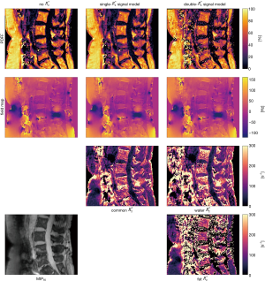
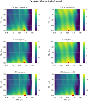
Figure 3 gives the result of the performed Cramér-Rao analysis and extends the result from (11) from a three-echo signal of a single-peak fat model without $R_2^{*}$ -relaxation to the common case of a six-echo sampling of a multi-peak fat model with common $R_2^{*}$ . The Monte-Carlo noise estimates for the NSA of all estimated parameters closely follow the theoretical CRLBs demonstrating consistency between the parameter estimation scheme, the Cramér-Rao simulation and literature.

Figure 3 Cramér-Rao lower bounds with Monte-Carlo estimates of parameter noise in a single-$R_2^{*}$ water-fat model. Experimental setting is defined by: number of echoes N_TE=6, first echo time TE₁ =1 ms, echo spacing ∆TE =1 ms, B₀ =3 T, $R_2^{*}$ =5 s⁻¹, field map ω/2π =10 Hz. The Monte-Carlo simulation was performed with 10⁵ independent noise realizations with signal-to-noise-ratio, SNR =100. The result is an extension of (11) from a single-fat-peak model without $R_2^{*}$ -decay to a multi-peak fat model (26) with a single $R_2^{*}$ . The agreement of the Monte-Carlo simulation with the theoretical number of signal averages (NSA) validates the consistency of the parameter estimation Algorithm 1 and the general Fisher information from Eq. [11].

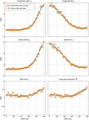
Figure 4 displays anatomical maps for uncertainty quantification of the parameter maps in the spine dataset from Figure 2. Assuming the estimated parameter maps as the true tissue parameters, the noise estimates are computed in each voxel for all models via Eq. [20]. The same noise behavior than in the theoretical assessment in Figure 3 can be observed: parameters containing fat magnitude and phase information are best estimated in lower fat fraction regions (compare to Figure 2), while in regions with high fat fraction, water parameters show higher NSA. The field map and relaxation rate estimates are not largely affected by different underlying fat fraction.

Figure 4 Anatomical maps showing estimated parameter uncertainty calculated as the Cramér-Rao lower bounds on the NSA noise measure for the estimated parameters from Figure 2, which are assumed to be the true underlying tissue parameters. Comparison of tissues with different proton density fat fraction (PDFF) is in agreement with theoretical results from Figure 3. For reference the maximum intensity projection across echo times (MIP_TE) is shown in the lower left corner.

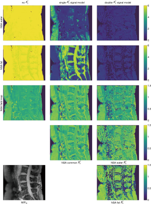
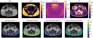
Figure 5 shows the capability of the generalized formulation to generate parameter maps for more complex models, like the fatty acid composition model, by only changing the constraint matrices as input for the implemented parameter estimation functions. While in the top row of subplots in Figure 5 the quantitative parameters common for the standard single-$R_2^{*}$ and the fatty acid composition model are compared, the lower row shows the derived additional quantitative parameter maps Eq. [24], with complementary information about fatty acid composition.

Figure 5 Quantitative parameter maps estimated with a more complex water-fat model describing additional fatty acid composition parameters. Experimental setting is defined by a monopolar time-interleaved multi-gradient-echo sequence with parameters: TR =24 ms, number of echoes N_TE =20 in two interleaves, TE₁ =1.5 m, ∆TE =1.0 ms, B₀ =3 T, flip angle =5°, bandwidth =961.5 Hz/pixel, FOV = (400×300×140) mm³, 2.0 mm isotropic resolution, SENSE factor =2.5 and scan time =3 min 8 sec. The dataset of 20 acquired echoes in the gluteal fat region allows to solve for a set of constraints matrices that include 12 independent parameters. Top row: maximum intensity projection over echo times, proton-density fat fraction, field map and common $R_2^{*}$ . Bottom row: parameter maps for additional tissue fat properties in the gluteal region. Values are in close agreement with previous studies (2,10,27).

In the Supplementary Materials we also gave an example for optimal echo time selection in terms of signal-to-noise ratios in the estimates shown in Figure S1.

Figure S1 Cramér-Rao lower bounds for NSA of parameter estimates in a single-$R_2^{*}$ water-fat model. Simulated experimental setting is defined by: number of echoes N_TE =6, first echo time TE₁ = 1 ms, echo spacing TE₁= 1 ms, ∆TE =1 ms, PDFF =30%, $R_2^{*}$ = 5 s⁻¹, field map ω/2π =10 Hz. The result is an extension of Reference (11) from a single-fat-peak model without $R_2^{*}$ -decay to a multi-peak fat model. Reference (26) with a single $R_2^{*}$ . Red markers indicate the first ten simulation points with maximized NSA.

Discussion

In this work, we developed a generalized formulation for the processing of multi-echo gradient-echo MR signals of multiple chemical species. We demonstrated how the developed signal analysis framework allows parameter estimation and noise performance analysis over a broad range of signal models that have the form of a weighted sum over complex exponentials, whose phase terms depend linearly on the echo time. The main result of the present study is the demonstration of the abundance of parameter estimation techniques that can be derived from the developed framework by changing simple input matrices. Therefore, the value and novelty of the presented work lie within the generality of the method across multiple different signal models rather than re-implementation of each specific signal model.

Generalized formulation

The main advantage of the proposed framework is the abstraction of model-specific relations between estimation parameters into a matrix formulation. The constraint matrices select the derivatives of the general signal model and describe how the model varies with each property of the present chemical species. The model Jacobian, the combined model derivatives, allows to not only derive general mathematical results like the generalized FIM Eq. [11], but also to develop programming code reusable for parameter estimation in the whole signal model class of summed complex exponentials. These two, computational and mathematical, abstraction benefits to handle a large class of signal models for parameter estimation or optimal experimental design are demonstrated in Figure 2 and the noise performance analysis in Figure 3.

Given a signal model of interest, one can follow three steps to apply the presented parameter estimation and noise performance analysis analogously to the example for the single-$R_2^{*}$ model Eq. [15]: (I) reformulate the signal model to the general form of a weighted sum of complex exponentials with time-linear arguments, Eq. [1]; (II) identify the variable mappings between original formulation and the general one together with the parameter constraints in the form of indicator functions for each parameter type; (III) translate the indicator functions to M × M matrices and remove any zero-columns.

As a consistency check one can compare the number of columns of all resulting rectilinear constraint matrices being equal the number of unknowns in the model. The constraint matrices are then input to the presented generalized methods.

Formulation validation and testing

To show the validity and generality of the proposed methods, we followed two motives.

First, the intrinsic consistency between the FIM-based noise analysis and the parameter estimation was tested in numerical simulations and Monte-Carlo and in vivo parameter estimations. Figure 3 demonstrates how the proposed formulation can reproduce established results from water-fat imaging literature. When no parameter relations are incorporated, the noise analysis is identical to previous results in MR spectroscopy literature (30,31). Similar to previous studies in water-fat separation, like for example by Pineda et al. (11), the comparison between the theoretical NSAs, here computed with the generalized FIM, and the implemented estimation algorithm in independently generated noisy signals shows the consistency between the noise analysis and the parameter estimation in the generalized formulation, exemplary for a six-echo sampling and a multi-fat-peak single- model.

Second, we showed reproducibility of established results with the generalized formulation in a subset of signal models previously studied in literature, primarily in water-fat imaging. Besides signal models with lower number of parameters, the more complex water-fat signal model to compute fatty acid composition parameters can similarly be represented as a set of constraint matrices. Figure 5 demonstrates how the proposed generalized formulation allows flexible formulation of the parameter estimation algorithm by choosing the corresponding constraint matrix inputs. The resulting fatty acid composition parameters are in close agreement with previous studies (2,10,27).

Limitations

The validity and versatility of the proposed generalized formulation could be demonstrated in this work, however, the formulation and the present study has some limitations.

First, the utilized constraint matrices are only able to encode linear parameter relations. While scaling between parameters, as e.g., the fat peak amplitudes in the magnitude constraint matrix, are direct elements in the constraint matrices, constant offsets between different parameters, as e.g., for a priori chemical shifts between fat peak resonance frequencies, are described by initial values in the parameter estimation algorithm. Higher order relations between different model parameters are not part of the generalized formulation.

Second, the generalized formulation is only suitable for the complex signal models in the class of summed exponentials up to now. The exponential arguments are only linear in the echo times and higher orders were not considered.

Third, it is often desirable to be able to constrain the phases ϕ of multiple chemical species to be equal. While the formulation naturally allows for these phase constraints, the Algorithm 1 in its current form does not lead to fully phase constraint results as the update of the linear magnitude parameters ϱ does not enforce their realness, only the phase updates are constrained. While this feature was not used in this study, the realness-enforcing algorithmic update of the linear parameters can be implemented according to the update step in (32).

Fourth, in practice the phase of the measured signal may sometimes be discarded due to possible phase errors of various sources. The resulting magnitude-based signal models are not described by the developed generalized formulations in this work, however the same concept of capturing parameter relations in matrix form are applicable considering the different noise distribution in the signal magnitude.

Free software/reproducibility research

The computer programs to implement the algorithms described above were developed in the Python programming language (Anacoda distribution of Python 3.6, https://www.anaconda.com). We made extensive use of the numpy, scipy, and numba module, which allowed for machine compiled and parallelized code execution ready for practical MRI applications with large (3D) multi-echo datasets. The developed computer programs used the data-structure of the ISMRM fat-water toolbox and are fully compatible with other routines within the ISMRM fat-water toolbox. Therefore, the presently developed software routines can be considered as an extension of the ISMRM toolbox allowing the adoption of signal models not included in the original ISMRM fat-water toolbox (12). To adhere to the idea of reproducible research, all code is freely available at the URL (https://github.com/maxdiefenbach/MR_CSS/) together with the scripts to generate all Figures from this publication.

Conclusions

We developed a formulation for multi-echo gradient-echo-based chemical species separation which allows to generalize gradient-based optimization algorithm development for the class of signal models described by a weighted sum of complex exponentials with phase terms linear in the echo time.

Acknowledgments

Funding: The present work was supported by the European Research Council (grant agreement No 677661, ProFatMRI). This work reflects only the authors view and the EU is not responsible for any use that may be made of the information it contains. The authors also acknowledge research support from Philips Healthcare.

Footnote

Conflicts of Interest: The authors have no conflicts of interest to declare.

Open Access Statement: This is an Open Access article distributed in accordance with the Creative Commons Attribution-NonCommercial-NoDerivs 4.0 International License (CC BY-NC-ND 4.0), which permits the non-commercial replication and distribution of the article with the strict proviso that no changes or edits are made and the original work is properly cited (including links to both the formal publication through the relevant DOI and the license). See: https://creativecommons.org/licenses/by-nc-nd/4.0/.

References

1. Reeder SB, Wen Z, Yu H, Pineda AR, Gold GE, Markl M, Pelc NJ. Multi-Coil Dixon Chemical Species Separation with an Iterative Least-Squares Estimation Method. Magn Reson Med 2004;51:35-45. [Crossref] [PubMed]
2. Berglund J, Ahlström H, Kullberg J. Model-Based Mapping of Fat Unsaturation and Chain Length by Chemical Shift Imaging-Phantom Validation and in vivo Feasibility. Magn Reson Med 2012;68:1815-27. [Crossref] [PubMed]
3. Alonso-Ortiz E, Levesque IR, Pike GB. MRI-Based Myelin Water Imaging: A Technical Review. Magn Reson Med 2015;73:70-81. [Crossref] [PubMed]
4. Wiesinger F, Weidl E, Menzel MI, Janich MA, Khegai O, Glaser SJ, Haase A, Schwaiger M, Schulte RF. Ideal Spiral CSI for Dynamic Metabolic MR Imaging of Hyperpolarized [1-13c]pyruvate. Magn Reson Med 2012;68:8-16. [Crossref] [PubMed]
5. Wang Y, Liu T. Quantitative Susceptibility Mapping (QSM): Decoding MRI Data for a Tissue Magnetic Biomarker. Magn Reson Med 2015;73:82-101. [Crossref] [PubMed]
6. Hernando D, Liang ZP, Kellman P. Chemical Shift-Based Water/fat Separation: A Comparison of Signal Models. Magn Reson Med 2010;64:811-22. [Crossref] [PubMed]
7. Bydder M, Yokoo T, Hamilton G, Middleton MS, Chavez AD, Schwimmer JB, Lavine JE, Sirlin CB. Relaxation Effects in the Quantification of Fat Using Gradient Echo Imaging. Magn Reson Imaging 2008;26:347-59. [Crossref] [PubMed]
8. Yu H, Shimakawa A, McKenzie CA, Brodsky E, Brittain JH, Reeder SB. Multi-Echo Water-Fat Separation and Simultaneous R2* Estimation with Multi-Frequency Fat Spectrum Modeling. Magn Reson Med 2008;60:1122-34. [Crossref] [PubMed]
9. Peterson P, Månsson S. Fat Quantification Using Multi-Echo Sequences with Bipolar Gradients: Investigation of Accuracy and Noise Performance. Magn Reson Med 2014;71:219-29. [Crossref] [PubMed]
10. Schneider M, Janas G, Lugauer F, Hoppe E, Nickel D, Dale BM, Kiefer B, Maier A, Bashir MR. Accurate Fatty Acid Composition Estimation of Adipose Tissue in the Abdomen Based on Bipolar Multi-Echo Mri. Magn Reson Med 2019;81:2330-46. [Crossref] [PubMed]
11. Pineda AR, Reeder SB, Wen Z, Pelc NJ. Cramér-Rao Bounds for Three-Point Decomposition of Water and Fat. Magn Reson Med 2005;54:625-35. [Crossref] [PubMed]
12. Hu HH, Börnert P, Hernando D, Kellman P, Ma J, Reeder S, Sirlin C. ISMRM Workshop on Fat-Water Separation: Insights, Applications and Progress in MRI. Magn Reson Med 2012;68:378-88. [Crossref] [PubMed]
13. Liu T, Wisnieff C, Lou M, Chen W, Spincemaille P, Wang Y. Nonlinear formulation of the magnetic field to source relationship for robust quantitative susceptibility mapping. Magn Reson Med 2013;69:467-76. [Crossref] [PubMed]
14. Yu H, McKenzie CA, Shimakawa A, Vu AT, Brau AC, Beatty PJ, Pineda AR, Brittain JH, Reeder SB. Multi-echo reconstruction for simultaneous water-fat decomposition and T2* estimation. J Magn Reson Imaging 2007;26:1153-61. [Crossref] [PubMed]
15. Karampinos DC, Yu H, Shimakawa A, Link TM, Majumdar S. Chemical shift-based water/fat separation in the presence of susceptibility-induced fat resonance shift. Magn Reson Med 2012;68:1495-505. [Crossref] [PubMed]
16. Reeder SB, Bice EK, Yu H, Hernando D, Pineda AR. On the performance of T2* correction methods for quantification of hepatic fat content. Magn Reson Med 2012;67:389-404. [Crossref] [PubMed]
17. Golub G, Pereyra V. Separable Nonlinear Least Squares: The Variable Projection Method and Its Applications. Inverse Probl 2003;19:R1-R26. [Crossref]
18. Reeder SB, Pineda AR, Wen Z, Shimakawa A, Yu H, Brittain JH, Gold GE, Beaulieu CH, Pelc NJ. Iterative Decomposition of Water and Fat with Echo Asymmetry and Least-Squares Estimation (ideal): Application With Fast Spin-Echo Imaging. Magn Reson Med 2005;54:636-44. [Crossref] [PubMed]
19. Hernando D, Haldar JP, Sutton BP, Ma J, Kellman P, Liang ZP. Joint Estimation of Water/fat Images and Field Inhomogeneity Map. Magn Reson Med 2008;59:571-80. [Crossref] [PubMed]
20. Hernando D, Kellman P, Haldar JP, Liang ZP. Robust Water/fat Separation in the Presence of Large Field Inhomogeneities Using a Graph Cut Algorithm. Magn Reson Med 2010;63:79-90. [PubMed]
21. Berglund J, Johansson L, Ahlström H, Kullberg J. Three-Point Dixon Method Enables Whole-Body Water and Fat Imaging of Obese Subjects. Magn Reson Med 2010;63:1659-68. [Crossref] [PubMed]
22. Berglund J, Skorpil M. Multi-Scale Graph-Cut Algorithm for Efficient Water-Fat Separation. Magn Reson Med 2017;78:941-9. [Crossref] [PubMed]
23. Cui C, Shah A, Wu X, Jacob M. A Rapid 3d Fat-Water Decomposition Method Using Globally Optimal Surface Estimation (R-GOOSE) Magn Reson Med 2018;79:2401-7. [Crossref] [PubMed]
24. Scharf L, McWhorter L. Geometry of the Cramér-Rao Bound. Victoria, BC, Canada: IEEE Sixth SP Workshop on Statistical Signal and Array Processing, 1992:5-8.
25. Ruschke S, Eggers H, Kooijman H, Diefenbach MN, Baum T, Haase A, Rummeny EJ, Hu HH, Karampinos DC. Correction of Phase Errors in Quantitative Water-Fat Imaging Using a Monopolar Time-Interleaved Multi-Echo Gradient Echo Sequence. Magn Reson Med 2017;78:984-96. [Crossref] [PubMed]
26. Hamilton G, Yokoo T, Bydder M, Cruite I, Schroeder ME, Sirlin CB, Middleton MS. In vivo Characterization of the Liver Fat 1H MR Spectrum. NMR Biomed 2011;24:784-90. [Crossref] [PubMed]
27. Peterson P, Månsson S. Simultaneous Quantification of Fat Content and Fatty Acid Composition Using MR Imaging. Magn Reson Med 2013;69:688-97. [Crossref] [PubMed]
28. Franz D, Diefenbach MN, Treibel F, Weidlich D, Syväri J, Ruschke S, Wu M, Holzapfel C, Drabsch T, Baum T, Eggers H, Rummeny EJ, Hauner H, Karampinos DC. Differentiating Supraclavicular From Gluteal Adipose Tissue Based on Simultaneous PDFF and T2* Mapping Using a 20-echo Gradient-Echo Acquisition. J Magn Reson Imaging 2019;50:424-34. [Crossref] [PubMed]
29. Liu CY, McKenzie CA, Yu H, Brittain JH, Reeder SB. Fat Quantification with Ideal Gradient Echo Imaging: Correction of Bias from T1 and Noise. Magn Reson Med 2007;58:354-64. [Crossref] [PubMed]
30. Nguyen H, Gahvari Z, Haldar J, Do M, Liang ZP. Cramér-Rao bound analysis of echo time selection for 1H-MR spectroscopy. Minneapolis, MN, USA: 31st Annual International Conference of the IEEE Engineering in Medicine and Biology Society, 2009.
31. Cavassila S, Deval S, Huegen C, Ormondt D, van , Graveron-Demilly D. Cramér-Rao Bounds: An Evaluation Tool for Quantitation. NMR Biomed 2001;14:278-83. [Crossref] [PubMed]
32. Bydder M, Yokoo T, Yu H, Carl M, Reeder SB, Sirlin CB. Constraining the Initial Phase in Water-Fat Separation. Magn Reson Imaging 2011;29:216-21. [Crossref] [PubMed]