

MR image reconstruction using deep learning: evaluation of network structure and loss functions
Introduction
MRI acceleration methods are widely used to shorten image acquisition time by under-sampling k-space. Parallel imaging methods such as GRAPPA (1) and compressed sensing (CS) (2) are state-of-the-art approaches that are routinely used. GRAPPA uses a fully-sampled k-space center region to train convolution kernels which are subsequently used to fill in missing k-space samples. However, a potential challenge of parallel imaging is that at high acceleration factors, the g-factor could result in significant noise amplification. The CS method takes advantage of the intrinsic sparsity of the data in a specific transform domain and random k-space sampling (incoherent point spread function) to remove noise-like image artifacts in the image. CS-MRI typically uses predefined and fixed sparsifying transforms, e.g., total variation (TV), discrete cosine transforms and discrete wavelet transforms (3). This can be extended to more flexible sparse representations learned directly from data using dictionary learning (4). However, CS-MRI is associated with challenges in finding appropriate regularizers for specific applications and manually tuning the hyperparameters, a time-consuming process that is difficult to standardize. In addition, the optimization process involves non-convex terms, so there is no guarantee of achieving a global minimum or even converging to a solution.
Recent advances in deep neural networks open a new possibility to solve the inverse problem of MR image reconstruction in an efficient manner. Deep learning-based approaches are well-developed in computer vision tasks such as image super-resolution (5-8), denoising and inpainting (9-12), while their application to medical imaging is still at a relatively early stage. For MR image reconstruction, these approaches typically learn the proper transformation between the input (zero-filled under-sampled k-space) and the target (the fully-sampled k-space) by minimizing a specific loss-function through a training process. Recently, a few different networks have been used to automate medical image reconstruction (13-21). Jin et al. (13) focused on CT reconstruction and proposed a Filter Back Projection Convnet (FBPConv) to reconstruct the CT data 1,000 faster than classic methods while preserving the image quality. Sandino et al. (16) trained a Unet architecture on 3D cardiac datasets and compared the results based on pixel-wise loss functions. Hammernik et al. (18) proposed variational network to learn the effective priors to accelerate the knee imaging and shorten the acquisition and reconstruction time. Schlemper et al. (19) proposed a novel deep cascade network for dynamic image reconstruction and showed superior performance of their network to CS-MRI. They used the data sharing layer to learn the spatiotemporal correlation of dynamic cardiac imaging data, which substantially improved the performance of their network. Hyun et al. (20) used a simplified Unet and proposed a k-space correction method to improve the performance of their network in MR reconstruction. Zhu et al. (21) used fully connected layers followed by a convolutional autoencoder to directly map the k-space data to the image domain.
Based on these published results, convolutional neural networks (CNNs) are able to learn more effective priors through supervised learning, compared to CS-MRI which employs simpler, fixed priors (typically based on sparse finite differences). Studies have mainly used pixel-wise cost functions for network training which can potentially reduce image sharpness. Some works have shown that high-quality images can be generated by using non-pixel-wise loss functions, such as perceptual loss (22,23).
For deep networks to be adopted for clinical MR reconstruction, several aspects need to be thoroughly evaluated. These include the various network architectures and effects of loss function choices on reconstruction performance. In addition, reconstructions need to be compared in the setting of prospectively under-sampled acquisitions rather than retrospective under-sampling.
In this work, we have implemented two state-of-the-art networks [Unet and residual network (Resnet)] using four different loss functions (pixel-wise L2, pixel-wise L1, structural dissimilarity (Dssim3) and perceptual loss). The performance was evaluated on cardiac imaging data from patients and volunteers with regard to signal-to-noise (SNR) (dB) and Structural Similarity Index (SSIM) in relation to qualitative scoring by board-certified cardiac radiologist. The purpose was to determine which approaches lead to improved CNN reconstructions for real time cardiac imaging. In vivo validation using prospectively under-sampled data was performed in 5 volunteers and one patient.
Methods
The MR image reconstruction problem can be formulated as an optimization problem. Suppose  is the reconstructed image and xz is the under-sampled k-space measurement. Fu is under-sampled Fourier encoding matrix. Since
  is an ill-posed linear system, the problem can be approached as an optimization of a data consistency term plus a regularization term:
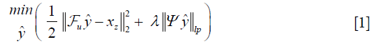
Where λ is a regularization parameter and Ψ is a sparsifying function. In general, the regularizer term includes lp norm (0≤p≤1) and predefined sparsifying functions may include finite difference or discrete wavelet functions. The global optimal is obtained by iterative algorithms such as alternating direction method of multipliers (ADMM) (24,25), or fast Iterative Shrinkage-Thresholding Algorithm (FISTA) (26). The ISTA methods apply an affine transformation followed by a non-linear coordinate-wise function (threshold sign function) in each iteration. This process is similar or at least analogues to a convolution layer in a neural network, which starts with an affine transformation and followed by a nonlinear activation function. Gregor et al. proposed a learned ISTA (LISTA) (27), which is based on training a feedforward network to estimate x* with 20 times less iteration than ISTA. This work not only paved the way for fast-CS approaches but also showed the possibility of applying deep learning based neural network to solve the ill-posed inverse problem.
In deep learning-based MR-reconstruction, the goal is to learn a function fcnn based on a large dataset that maps under-sampled, zero-filled data to fully sampled images by minimizing a loss function.
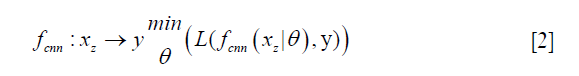
Where 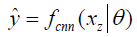 is the reconstructed image by CNN in a forward propagation with parameter θ. xz is under-sampled data and L is the loss function. The following loss functions were evaluated in this work:

where, H is the height (number of rows) of each 2D image, W is the width of the image, B is batch size, i.e. the number of images per batch, P is the number of patches for the Dssim3,  ,
,  are the ground truth image and the reconstructed image, respectively. The first two-loss functions {Eqs. [3,4]} are pixel-based loss functions, which depend on low-level pixel information only. The third loss function {Eq. [5]} penalizes Dssim between the two images. Lpercep (VGGi) represents the Euclidean distance between the produced features of imported y and
  to VGG-16 (28) in the first layer of the ith block after activation. As shown in Figure 1, in each epoch, the target image (y) and the
 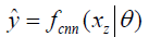 flow to the VGG-16 network independently, and the optimizer tries to minimize the weighted (λw) mean squared error of perceptual loss. The weighted perceptual loss function used in this study is described in Eq. [7]:
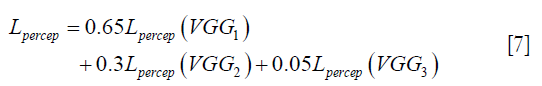
 ) and ground truth image (y) are calculated. A cost function is shown in Eq. [7] is calculated based on a weighted mean squared error in the feature space and is used in the backpropagation stage.
Similar loss functions have been used for super resolution reconstruction (22) and Eq. [7] can be regarded as one example from a family of perceptual loss functions that imparts higher importance to the first layers in capturing image features. We empirically assign more weight to the b1c1 layer of the VGG-16 than to the other two layers, because the extracted features are expected to progressively become more abstract in the deeper layers.
Finally, CNN training requires the cost functions to be minimized through the well-known backpropagation algorithm, which is defined by the chain rule:
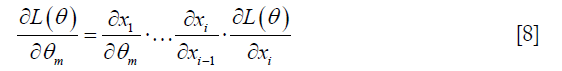
Index of x equals to layer number. For instance, xi stands for the last layer’s output.
Network architectures and training
The convolutional Unet has been used previously to solve inverse problems in computed tomography and MRI reconstruction (13,16,20,29). In general, it consists of two paths: (I) the contracting path, which contains a number of down-sampling stages; (II) the expanding path, which includes a number of up-sampling stages. In order to preserve high-level features, it consists of dense connections from the early stages to the later stages of the network. A version of the Unet architecture containing 1.3 million trainable parameters is shown in Figure 2A.

Figure 2B shows an example of Resnet CNN structure. It consists of several residual blocks (RBs) followed by two convolution layers. Inside each RB, there are two convolutional layers by batch normalization and ReLU activation. Residual connections facilitate the training process of the deep neural networks and is effective in removing the aliasing artifacts (13,30,31). The number of trainable parameters for this network with 4 (n:32,n:3×3) RBs is approximately 100,000, which is 13 times less than a simplified version of convolutional Unet.
For training the Unet and the Resnet, we used the loss functions described in Eqs. [3-6] and the RMSPropOptimizer with a learning rate of 0.001, weight decay of 0.9 and mini-batch size of 32 at each epoch. We empirically chose to perform 100 epochs for both networks based on the convergence of validation loss. In initial experiments, we observed for a learning rate of 0.001, that there was no noticeable reduction in validation loss beyond 100 epochs.
Network training was implemented in Tensorflow on Windows, NVIDIA TITAN Xp and required approximately 4–6 h.
Quantitative and qualitative image analysis metrics
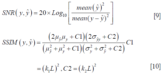
To quantify the reconstruction error, SNR (dB) and SSIM were used. SNR and SSIM were calculated based on the Eqs. [9,10]:
Where  and
and  are the local means, standard deviations, and cross-covariance for reconstructed and ground truth images. C1 and C2 are two variables to stabilize the division with weak denominator. L is the dynamic range of the pixel values and k1 =0.01, k2 =0.03 are constant values. Local operations (local mean or variance) were calculated in a 3×3 rectangle box.
To qualitatively compare the performance of the networks and loss functions in image reconstruction, blinded image quality comparison by using a 1–5 ranking system were performed with an expert radiologist. Table 1 summarized criteria for the scoring.

Full table
MR data acquisition
The study was approved by our institutional review board and each subject provided written informed consent. Three types of cardiac datasets were included in this study:
Real-time cardiac imaging using a continuous balanced steady state free precession (bSSFP) sequence with a surface coil array on a 1.5T MRI scanner (Avanto Fit, Siemens Healthcare; Erlangen, Germany) was performed in 5 healthy volunteers. For each volunteer, 200 fully sampled images were acquired continuously (temporal resolution =333 ms/cardiac frame) in the cardiac short-axis (SA) view during free breathing without ECG-gating;
Conventional k-space segmented breath-held cardiac cine images from 48 patients who underwent clinically indicated cardiac MRI exams were retrospectively included in this work;
Real time cardiac cine data with prospective 4X k-space under-sampling were acquired in 5 additional healthy volunteers and 1 additional patient for network testing.
Network training and testing based on retrospectively under-sampled data
The network was trained and validated based on Datasets 1 and 2. The k-space data from the 48 patient images were retrospectively under-sampled by a typical GRAPPA under-sampling pattern (4×, 22 auto-calibration lines) and zero-filled images were produced using inverse 2D FT. Each individual image was normalized linearly to have an intensity between 0 and 1 and matrix size adjusted to 192×128. The real time cardiac cine data from the 5 volunteers were also retrospectively under-sampled in a similar fashion. The 5 healthy volunteers and 48 patient datasets were split randomly into 3 different sets including: (I) training set (3 healthy volunteers +24 patients); (II) validation set (1 healthy volunteer +6 patients); (III) test set (1 healthy volunteer +18 patients). For the training set, among 20,000 images, 2,000 images were selected that included a large diversity of cardiac data with regard to anatomy and imaging orientation. For the validation set, in each epoch, 500 random images from the 6,000-image validation dataset were selected. The test set included all of the images acquired in the volunteer and the 18 patients in the test set (III).
The following evaluations were performed on the test set (III):
- We evaluate the loss functions using the Unet, which is representative of existing CNN architectures used in MRI reconstruction;
- Using the preferred loss function from part (i) we implemented a new Resnet architecture to compare with the Unet and explored key parameters for this network;
- Statistical comparison between the performance of the various loss functions and network architectures were performed according to the aforementioned metrics in qualitative image quality scoring and SNR/SSIM measures.
Testing based on prospectively under-sampled data
To further demonstrate the performance of our technique, we also compared the performance of the Unet and Resnet architectures based on qualitative image quality scoring using our prospectively under-sampled data in Dataset 3 to mimic a more realistic clinical scenario. The under-sampling trajectory used in Dataset 3 was the same as the retrospective under-sampling trajectory used for Datasets 1 & 2.
Results
To evaluate the performance of the four loss functions (L1, L2, Dssim3, Perceptual loss), we performed image reconstructions using the test set data based on the Unet shown in Figure 2A. As can be seen in Figure 1, the perceptual loss function VGG-16 is a pre-trained network that minimizes the mean square error in the feature space. Our perceptual loss function uses features extracted from the first three layers of the VGG-16 [bic1 (i =1,2,3)] according to Eq. [7]. Figure 3 shows representative reconstruction results of the Unet based on the four loss functions from a randomly chosen patient from our study. The reconstruction based on perceptual loss function produced considerably sharper boundaries for the anatomical structures and was closest to the ground truth.

For the Resnet structure, the number of RBs included in the network has significant impact on the image quality. In order to find a proper number of RBs for Resneti [32, 3], different number of RBs ranging from 2 to 7 was tested. In this step, all the Resneti [32, 3] networks were trained using perceptual loss function. To have a fair comparison, all other parameters related to optimizer were fixed. Figure 4 shows the reconstruction results for Unet (perceptual) and the Resneti [32, 3] networks with 2–4 RBs. The image reconstruction of Resneti [32, 3] with 2 or 3 RBs provided sub-optimal results due to residual noise and image blurring. The Resneti [32, 3] reconstruction with 4 RBs was similar to the Unet reconstruction; however, as marked with blue arrow, certain subtle details were better recovered with Unet. Regions pointed to by the red arrows were not recovered well by either Resneti [32, 3] or Unet, when compared with ground truth. For the remainder of the work, all Resnet is Resnet4 Resneti [32, 3], i.e., Resnet with 4 RBs, and 32 convolution kernels of size 3×3.

To identify any statistically significant differences in the image quality of Unet- and Resnet-based reconstructions using various loss functions, an experienced clinical MRI evaluator subjectively assessed the image quality using a 1–5 ranking system. We randomly chose 25 datasets from our study data, each dataset including 5 images reconstructed using five techniques: (I) Unet with perceptual loss function; (II) Resnet using perceptual loss function; (III) Unet with Dssim loss function; (IV) Unet with L1 loss function; (V) Unet with L2 loss function. During the evaluation session, the evaluator was presented one dataset at a time with the order of the five images randomized and blinded to the evaluator. The evaluator was asked to rank the five images from 1–5, 1= best subjective image quality. Figure 5A shows the ranking score distributions for each of the five reconstruction techniques. To asses if the difference was significant, null hypothesis is assumed that the rank distribution of groups is same. Null hypothesis is rejected significantly (P<0.05) by applying Friedman’s two-way analysis (32) on the rank scores of different groups. Paired comparisons between the 5 techniques are reported in Figure 5B, which shows that the Unet with perceptual loss had significantly (P<0.05) better ranking than the remaining three Unet techniques with L1, L2 and Dssim loss functions, respectively. There was no statistically significant difference between Unet with perceptual loss and the Resnet with perceptual loss. Figure 5C graphically demonstrates the statistical analysis results, with yellow lines indicating statistically significant differences.

To show the potential utility of the networks in real clinical scanning scenario, Figure 6 demonstrates representative prospective reconstruction results from 4 healthy volunteers using Unet (perceptual) and Resnet4-Perceptual [32, 3]. The data was prospectively acquired with k-space under-sampling and reconstructed using the networks (which had been trained on retrospectively acquired data). The prospective data was acquired using a bSSFP sequence with 4X k-space under-sampling. The performance of the Unet and Resnet in the reconstruction of prospectively under-sampled data was diagnostically acceptable based on radiologic scores.

Tables 2-4 summarizes quantitative metrics for reconstruction results of the test set using Unet and Resnet with the 4 cost functions studied in this work. The normality test shows that the SNR and SSIM metrics were not normally distributed. The results show that the conventional pixel-wise loss functions (L1, L2) and Dssim are associated with higher SNR and SSIM than perceptual loss. However, the subjective image quality ranking by radiologist (Figure 5) and the visual assessment (Figure 3) favor the perceptual loss function.

Full table

Full table

Full table
Discussion
Neural networks or any supervised learning algorithms create the output based on pre-defined cost functions. Training the network based on pixel-wise loss functions such as L2, L1, and even Dssim (patch-wise loss function) produces a blurry image in reconstruction tasks. As can be seen in Figure 3, reconstruction results for Unet (L1), Unet (L2) and Unet (Dssim) appear blurry in comparison to Unet (perceptual). This is because pixel-wise loss functions remove part of image texture information and produce blurry output. For the region with flat signal intensity marked by a blue star, the output of Unet (L2) and Unet (L1) was contaminated with the splotchy artifact. The Unet (Dssim) and Unet (perceptual) maintained the constant signal intensity that is free of splotchy artifacts. Subjective image quality ranking results in Figure 5A is consistent with this observation. Based on results in Tables 2-4, Unet (Dssim) had the highest SSIM and Unet (L1) had the highest SNR among the techniques compared. However, these images had significantly lower subjective image quality ranks in comparison to Unet (perceptual). This disagreement exists because the SNR and SSIM metrics evaluate aspects of the images that may be different from how a radiologist visually perceive the images. One could argue that perceptual loss could be more correlated with visual image quality scoring. In order to develop and validate a more appropriate quantitative evaluation parameters that are better correlated with visual image quality scoring, a separate cost network could be designed and trained based on visual image quality scores. However, development of such an image quality evaluation network is beyond the scope of the current work.
Our results in Figure 5 and Tables 2-4 emphasizes the importance of choosing appropriate loss functions in training the network. In this work, the perceptual loss function based on the pre-trained VGG-16 network performed better than the other three pixel-wise loss functions. Future research is warranted to develop and train more advanced networks for the loss function.
The Resnet in the study had less than 0.1 million trainable parameters, but could produce comparable results to Unet with >1.3 million trainable parameters. As reported graphically in Figure 5C, the difference between subjective image quality ranks using the Resnet4 [32, 3] with perceptual loss and the Unet with perceptual loss was not statistically significant. Both networks could be implemented in online MR-reconstruction applications. In Figure 4, certain details in the ground truth image as marked with red arrow and green circle was not recovered completely with either Unet or Resnet. This issue could be possibly related to regular parallel imaging- type k-space under-sampling patterns. Using variable density under-sampling pattern may improve the reconstruction results further. Such a variable density pattern may be better applied in 3D acquisitions due to the flexibility of designing the sampling pattern in both phase encoding and slice encoding directions. As mentioned in Figure 4 and marked with the blue arrow, Unet preserves some subtle details better than Resnet4. This could be due to the larger of trainable parameters in the Unet and more importantly the dense connections. The dense connections helped the network to reuse the extracted features from previous layers. Although in the Resnet architecture, there are residual connections, the difference seems related to the concatenation and global connection paths in the Unet.
By increasing the number of RBs from 2 to 7, the validation loss of Resnet with perceptual loss reduced from 0.1731 to 0.1366. We showed the results for Resnet with 2 to 4 RBs, because we observed no significant reduction of the validation loss of Resnet with 4 blocks (0.1376) to Resnet with 7 blocks (0.1366). It is important to mention that, the number of kernels within each block was fixed to 32. Increasing the number of kernels may further improve the reconstruction performance, although it would also increase the number of trainable parameters.
The number of epochs for training the network was selected based on validation loss. Due to several experiments, we observed for learning rate =0.001, the training process should be stopped at 100 epochs, because, after 100 epochs, there were no noticeable reductions in validation loss. In this study, we focus on achieving clinically accepted results by using a simple version of Resnet. It is beyond the scope of the current study to further optimize certain aspects of the network, including: (I) number of kernels of each block; (II) using dense connection instead of residual connection; (III) using multiscale filters inside each block; (IV) using a gated version of RBs. These optimizations have been studied in computer vision tasks (33-36), but not specially studied in image reconstruction problems.
In this work, temporal information was not considered and only space domain information was used. It is possible to use recurrent CNNs to exploit the temporal information. Nevertheless, adding an additional temporal dimension to CNNs could significantly increase the complexity of the network and may result in challenges in training. Development and evaluation of such strategies require a separate study.
As shown in Figure 6, the performance of the Unet and Resnet in the reconstruction of prospectively under-sampled data was diagnostically acceptable based on the radiologic scores. Based on our observation, prospective results by a small margin have inferior quality in comparison to retrospective results. Such small differences show that the trained network was robust to the changes in the dataset. It is worth to note that previous studies in deep learning-based image reconstruction almost always train and test the network retrospectively. In this study, by changing the sampling pattern of the pulse sequence, performance of networks in the real prospectively accelerated cardiac exam is shown. Further investigation should be performed to understand the difference between prospectively under-sampled data and retrospectively under-sampled data. With a good understanding of the difference, one could change training data to mimic prospective undersampled data, therefore, fine-tuning the network and improving further the performance of the network for prospective reconstruction tasks.
Conclusions
Deep learning-based image reconstruction help to achieve a 4-fold acceleration in 2D cardiac imaging, prospectively. The images reconstructed using the network based on perceptual loss function can generate the best image quality compared to the other loss function (L1, L2, and SSIM), despite not generating the best SNR or SSIM score. Resnet used in this work generate reconstructed image with the similar quality compared to that by Unet while required only 8% of the trainable parameters needed for Unet.
Acknowledgments
Funding: The study was supported by National Institutes of Health under award numbers R01HL127153.
Footnote
Conflicts of Interest: The authors have no conflicts of interest to declare.
Ethical Statement: The study was approved by University of California, Los Angeles, Institutional Review Board and each subject provided written informed consent.
References
- Griswold MA, Jakob PM, Heidemann RM, Nittka M, Jellus V, Wang J, Kiefer B, Haase A. Generalized autocalibrating partially parallel acquisitions (GRAPPA). Magn Reson Med 2002;47:1202-10. [Crossref] [PubMed]
- Lustig M, Donoho DL, Santos JM, Pauly JM. Compressed sensing MRI. IEEE Signal Process Mag 2008;25:72-82. [Crossref]
- Lustig M, Donoho D, Pauly JM. Sparse MRI: The application of compressed sensing for rapid MR imaging. Magn Reson Med 2007;58:1182-95. [Crossref] [PubMed]
- Ravishankar S, Bresler Y. MR Image Reconstruction From Highly Undersampled k-Space Data by Dictionary Learning. IEEE Trans Med Imaging 2011;30:1028-41. [Crossref] [PubMed]
- Dong C, Loy CC, He K, Tang X. Image Super-Resolution Using Deep Convolutional Networks. IEEE Trans Pattern Anal Mach Intell 2016;38:295-307. [Crossref] [PubMed]
- Kim J, Lee JK, Lee KM. Accurate Image Super-Resolution Using Very Deep Convolutional Networks. 2016 IEEE Conference on Computer Vision and Pattern Recognition (CVPR). Available online: https://ieeexplore.ieee.org/document/7780551/
- Wang Z, Liu D, Yang J, Han W, Huang T. Deep Networks for Image Super-Resolution with Sparse Prior. Proceedings of IEEE International Conference on Computer Vision (ICCV). Available online: https://ieeexplore.ieee.org/document/7410407
- Cui Z, Chang H, Shan S, Zhong B, Chen X. Deep Network Cascade for Image Super-resolution. In: Fleet D, Pajdla T, Schiele B, Tuytelaars T. editors. ECCV 2014. Springer Nature, 2014:49-64.
- Xie J, Xu L, Chen E. Image Denoising and Inpainting with Deep Neural Networks. In: Pereira F, Burges CJC, Bottou L, Weinberger KQ. editors. Proccedings of Advances in Neural Information Processing Systems-volume 1. 2012:341-9.
- Jain V, Seung HS. Natural Image Denoising with Convolutional Networks. In: Koller D, Schuurmans D, Bengio Y, Bottou L. editors. Advances in Neural Information Processing Systems 21 - Proceedings of the 2008 Conference. 2008:769-76.
- Zhang K, Zuo W, Chen Y, Meng D, Zhang L. Beyond a Gaussian denoiser: Residual learning of deep CNN for image denoising. IEEE Trans Image Process 2017;26:3142-55. [Crossref] [PubMed]
- Chen Y, Pock T. Trainable Nonlinear Reaction Diffusion: A Flexible Framework for Fast and Effective Image Restoration. IEEE Trans Pattern Anal Mach Intell 2017;39:1256-72. [Crossref] [PubMed]
- Kyong Hwan Jin. McCann MT, Froustey E, Unser M. Deep Convolutional Neural Network for Inverse Problems in Imaging. IEEE Trans Image Process 2017;26:4509-22. [Crossref] [PubMed]
- Chen H, Zhang Y, Kalra MK, Lin F, Chen Y, Liao P, Zhou J, Wang G, Low-Dose CT. With a Residual Encoder-Decoder Convolutional Neural Network. IEEE Trans Med Imaging 2017;36:2524-35. [Crossref] [PubMed]
- Majumdar A. Real-time Dynamic MRI Reconstruction using Stacked Denoising Autoencoder. arXiv:1503.06383.
- Sandino CM, Dixit N, Cheng JY, Vasanawala SS. Deep convolutional neural networks for accelerated dynamic magnetic resonance imaging. Available online: http://cs231n.stanford.edu/reports/2017/pdfs/513.pdf
- Wang S, Su Z, Ying L, Peng X, Zhu S, Liang F, Feng D, Liang D. Accelerating magnetic resonance imaging via deep learning. Proccedings of IEEE 13th International Symposium on Biomedical Imaging (ISBI). Available online: https://ieeexplore.ieee.org/abstract/document/7493320/
- Hammernik K, Klatzer T, Kobler E, Recht MP, Sodickson DK, Pock T, Knoll F. Learning a Variational Network for Reconstruction of Accelerated MRI Data. Magn Reson Med 2018;79:3055-71. [Crossref] [PubMed]
- Schlemper J, Caballero J, Hajnal JV, Price AN, Rueckert D. A Deep Cascade of Convolutional Neural Networks for Dynamic MR Image Reconstruction. IEEE Trans Med Imaging 2018;37:491-503. [Crossref] [PubMed]
- Hyun CM, Kim HP, Lee SM, Lee S, Seo JK. Deep learning for undersampled MRI reconstruction. arXiv: 1709.02576.
- Zhu B, Liu JZ, Cauley SF, Rosen BR, Rosen MS. Image reconstruction by domain-transform manifold learning. Nature 2018;555:487-92. [Crossref] [PubMed]
- Johnson J, Alahi A, Li FF. Perceptual Losses for Real-Time Style Transfer and Super-Resolution. arXiv:1603.08155.
- Wu B, Duan H, Liu Z, Sun G. SRPGAN: Perceptual Generative Adversarial Network for Single Image Super Resolution. arXiv: 1712.05927.
- Yang Y, Sun J, Li H, Xu Z. Deep ADMM-Net for Compressive Sensing MRI. arXiv:1705.06869.
- Wang J, Shen HT, Song J, Ji J. Hashing for Similarity Search A Survey. 2014.
- Beck A, Teboulle M. A Fast Iterative Shrinkage-Thresholding Algorithm for Linear Inverse Problems. SIAM J Imaging Sci 2009;2:183-202. [Crossref]
- Gregor K, LeCun Y. Learning Fast Approximations of Sparse Coding. In: Fürnkranz J, Joachims T. editors. Proceedings of the 27th International Conference on International Conference on Machine Learning. 2010:399-406.
- Simonyan K, Zisserman A. Very Deep Convolutional Networks for Large-Scale Image Recognition. arXiv:1409.1556.
- Han Y, Yoo J, Kim HH, Shin HJ, Sung K, Ye JC. Deep learning with domain adaptation for accelerated projection‐reconstruction MR. Magn Reson Med 2018;80:1189-205. [Crossref] [PubMed]
- McCann MT, Jin KH, Unser M. Convolutional Neural Networks for Inverse Problems in Imaging: A Review. arXiv:1710.04011.
- Wu S, Zhong S, Liu Y. Deep residual learning for image steganalysis. Multimed Tools Appl 2018;77:10437-53. [Crossref]
- Forthofer RN, Lee ES, Hernandez M. Chapter 9: Nonparametric Tests. Biostatistics:: A guide to design, analysis, and discovery. Elsevier, 2007:249-68.
- Xie S, Girshick R, Dollár P, Tu Z, He K. Aggregated Residual Transformations for Deep Neural Networks. arXiv:1611.05431.
- Savarese PHP, Mazza LO, Figueiredo DR. Learning Identity Mappings with Residual Gates. arXiv:1611.01260.
- Huang G, Liu Z, van der Maaten L, Weinberger KQ. Densely Connected Convolutional Networks. arXiv:1608.06993.
- Zagoruyko S, Komodakis N. Wide Residual Networks. arXiv:1605.07146.

