

In vivo quantification of proton exchange rate in healthy human brains with omega plot
Introduction
Chemical exchange saturation transfer (CEST) MRI is an emerging endogenous molecular imaging technique whose contrast is produced through the transfer of selectively saturated protons from endogenous metabolites to bulk water. CEST MRI features high sensitivity and spatial resolution. Based on the abundance of the CEST-expressing metabolites in tissue, their proton exchange rate, the resonance frequency of their exchanging protons, and by varying the saturation parameters, CEST MRI can be tailored to image many different metabolites, including amide proton transfer (APT) (1), glycogen (2), glycosaminoglycans (3), brain glutamate (4), and glucose (5,6) with resolution down to the sub-millimeter range and high reproducibility (<3% of variation) (7).
The major proton exchanging sites in endogenous metabolites include amine (–NH2), amide (–NH), hydroxyl (–OH), and hydrosulfuric (–SH) groups. As a fundamental biophysical process, proton exchange plays important roles in producing MR imaging contrasts including T1- and T2- relaxations, chemical exchange saturation transfer, magnetization transfer (MT), and nuclear Overhauser enhancement (NOE). Imaging of proton exchange rate can also serve as indicator for changes in pH, temperature, or reactive oxygen species (8). Besides the importance of proton exchange in MRI, its quantification and imaging in vivo tissues has not yet been accurately achieved.
Omega plotting (9) provides a direct scheme to determine the proton exchange rate independently from the labile proton concentration. This technique was initially developed to measure the proton exchange rate of paramagnetic CEST (paraCEST) agents (10). In paraCEST agents, the resonance frequencies of labile protons are far off from the water resonance and hence their signal is not affected by the direct saturation (DS) of water protons (the “spillover” effect). For in vivo tissues, the proton exchange is however associated with endogenous diamagnetic CEST (diaCEST) metabolites (11). Unlike paraCEST, exchangeable protons in diaCEST agents resonate close to water, typically within 5 ppm (12). The small chemical shift of diaCEST agents comes as a disadvantage given that the acquired signal can be affected by the DS of bulk water. DS-corrected omega plots have been successfully implemented for kex mapping in solutions (13). It has been demonstrated that the accuracy of the modified omega plot analysis is greatly improved compared to the unmodified one, using both numerical simulations and experiments on solution phantoms (13). We believe it is necessary to investigate if removing DS effect may also help for the quantification of the exchange rate of in vivo tissues.
Furthermore, for in vivo tissues there may be many saturation transfer and exchanging proton species associated with various endogenous metabolites, resonating at any given frequency offset and exchanging at different rates. The omega plot developed on phantom studies (9), however, was derived to quantify the exchange rate of a single proton species. It is therefore necessary to extend the omega plot to a more general form by taking into account multiple species in vivo. In this study, we aim to implement and translate the omega plot method for in vivo mapping of proton exchange rates in human brains by taking into account the water DS effect and the multiple species under the in vivo conditions. Here we will expand the omega plot equation derivation for more than one saturation transfer sources, including macromolecules (the MT effect), metabolites with labile protons (the CEST effect), metabolites with exchange-relayed nuclear Overhauser effect (the NOE effect), etc. proton species that can exchange protons with bulk water.
Saturation transfer from multiple species
For a pool of solute protons undergoing continuous RF saturation and exchanging with another pool (i.e., water) at a rate fast relative to its relaxation rates (k≫R1 & R2), the reduction in magnetization can be calculated according to the Bloch-McConnell equations (9):
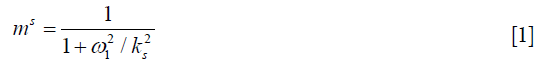
where  is the ratio of the protons’ final steady-state magnetization (
 ) over their initial equilibrium magnetization (
 ), ω1 = γB1 is the amplitude of the saturation RF pulse, and ks is the protons’ exchange rate.
This reduction of signal, the ‘saturation’, gets transferred from the protons of the solute i (si) to the bulk water pool. The rate of this saturation transfer exchange,  , depends on a number of factors: the exchange rate (
 ) between the solute pool and the water pool, the fraction of protons on the solute relative to water protons (
 ), and the signal from the solute protons (
 )
)

in which can be written as  , assuming there are vi exchanging protons in each molecule of solute si, and 2[w] is the molar concentration of water protons as there are two protons in each water molecule.
The magnetization of bulk water protons, mw, decreases due to the transferred saturation at the rate of

In the meantime, it recovers according to the longitudinal relaxation rate,  , at the rate of

At the steady state, longitudinal relaxation recovery balances with the saturation transfers as shown in Eq. [5]:

assuming there are n solute species contributing to the signal at the given saturation offset.
Reverting the water magnetization ratio to its steady-state and equilibrium values, i.e.,  , the above equation can be written as
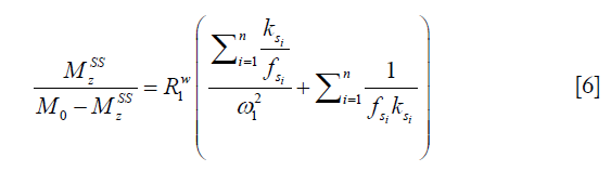
in which M0 and Mz are the Z-spectrum signals far from water resonance and at the metabolite resonance, respectively. This relation, which is a more generalized form of the omega plot equation, takes into account multiple solute species exchanging with water.
Eq. [6] indicates a linear relationship between the inverse of the Z-spectral signal intensity, (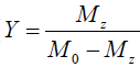 ), and the inverse of the square of saturation pulse power, (
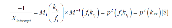
 ). In the Y vs. X plot (the omega plot) the X-axis intercept can provide a readout of the convoluted averages of the solutes’ exchanging rates:
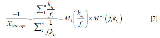
where M1 and M−1 are the arithmetic and the harmonic mean operator, respectively. In the case of single metabolite, the familiar omega plot readout, 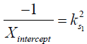 , is recovered.
Our derivation of the generalized omega plot equation indicates that for in vivo situations when many metabolites contribute to the saturation transfer signal, the omega plot still shows linear dependency to  , but the X-axis intercept indicates now a profile of the average saturation transfer exchanging rate of all the contributing metabolites:
Water DS correction
The Z-spectral signal used for the computation is not solely affected by proton exchange dependent mechanisms, such as CEST, MT, and NOE (14,15). It is also affected by the dominant water DS effect, particularly when the saturation offset is close to the water proton resonance, as in diaCEST imaging. The DS effect can thus contaminate the proton exchange rate quantification using the omega plot, especially for endogenous diaCEST metabolites.
Due to the presence of contralateral NOE effect in the reference signals in our Z-spectra the simple MT asymmetric analysis for removing DS and MT cannot be used. To improve the proton exchange rate quantification, one may try to mathematically remove the water DS contributions from the Z-spectrum. Lorentzian functions have been used to fit the Z-spectrum as a linear combination of multiple components (16). Variants of this method have already been employed in many studies, for instance, taking Z-spectrum as the sum of four (DS, Amide, Amine and NOE) (17), or five Lorentzian function (DS, MT, NOE, Amide and 2 ppm peak) (18). However, fitting with multiple Lorentzians is feasible mostly for Z-spectra collected at high field or with low saturation power B1.
In the present study, our goal was to map the proton exchange rates in healthy human brains at a clinical 3T scanner. Given that Z-spectra at 3T typically do not show prominent CEST and NOE peaks, we fitted each Z-spectrum with two Lorentzian functions, corresponding to DS and the residue spectrum (containing CEST, NOE, and the semi-solid MT), in order to remove the DS contribution. The residual signal, free from water DS, is then used for computing proton exchange rates maps of healthy human brains by the omega plot method.
Methods
Healthy volunteers (n=10, 22–25 years old, males and females) were recruited for MRI scanning. The study was approved by the institutional review board, and signed consent was obtained prior to all examinations. MR imaging of human brains was performed on a 3.0T GE MR750 scanner (GE Healthcare, Waukesha, WI) with a 32-channel head coil. T2-weighted images were used for the initial anatomical slice selection. Single-slice Z-spectral data were acquired from a middle brain slice parallel to the anterior commissure-posterior commissure (AC-PC) line. Sequence parameters were as follows: TR/TE =3,000/22.6 ms, field of view (FOV) =24×24 cm2, matrix =128×128, slice thickness =5 mm, number of excitations (NEX) =2, saturation power =1, 2, 3 & 4 µT, saturation duration =1,500 ms. The Z-spectral images were acquired using a single-shot fast low-angle shot (FLASH) readout (19). Each Z-spectrum contained 33 images acquired at these saturation offsets: +15.6, ±6, ±5, ±4.5, ±4, ±3.75, ±3.5, ±3.25, ±3, ±2.5, ±2, ±1.5, ±1, ±0.75, ±0.5, ±0.25, 0, and +39.1 ppm. The total scanning time for the Z-spectral data was 3 min 18 s.
To demonstrate that DS-corrected Z-spectra along with omega plot can be used to detect exchange rate variation, ex vivo protein solutions at different pH were studied. Phantoms containing 20% (w/w) bovine serum albumin (BSA) (Sigma-Aldrich Corp., St. Louis, MO, USA) protein solutions were freshly prepared in phosphate-buffered saline (PBS) (n=3) at room temperature with pH titrated to 6.2, 6.6, 7.0 & 7.4. MRI was carried out at a 9.4T preclinical Agilent MRI System (Agilent Technologies, Santa Clara, CA, USA) on a single slice with these parameters: FOV = 2×2 cm2, matrix = 128×128, slice thickness =3 mm, NEX =2. The Z-spectra were acquired with the same saturation powers, durations and offsets as in the human study.
Data analysis
Prior to the creation of the pixel-wise exchange rate maps, a number of processes were performed on the MRI data including: motion correction, interpolation of the Z-spectra, fitting of the Z-spectra to remove the DS peak, construction and fitting of the omega plot and quantification of saturation transfer exchanging rate. All these data analyses were performed in MATLAB (MathWorks, Natick, MA) with self-developed programs.
The motion artifacts due to involuntary head movements during the data acquisition were corrected by MATLAB’s intensity-based image registration routine “imregister”. In our procedure, at first the 39.1 ppm reference image from each CEST sequence was registered to that of B1=3 µT series (as the series acquired halfway through the study). In each series, the overall images intensity changes gradually as the saturation frequency shifts closer to the water resonance. To take into account these gradual changes, each image was registered to the previous adjacent image, which is assumed to have the most comparable intensity. This method is similar to a previous reported study (20).
In the fitting procedure, the Z-spectra within ±6 ppm range were normalized to the signal at +39.1 ppm. Z-spectra were then flipped to be 100×(1 − Mz/M0) and fitted to a sum of two Lorentzian functions, the first corresponding to the bulk water and the second to a sum of the remaining effects (mainly MTC from semi-solid components, CEST and NOE, overall, hereafter referred to as the DS-removed Z-spectrum), centered around 0 and −1.5 ppm respectively. The fitting function was:
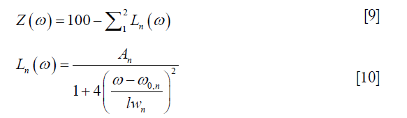
where ω is the frequency offset relative to water resonance, and A, ω0 and lw are respectively the amplitude, center frequency offset, and line-width of each peak. These parameters were fitted iteratively using MATLAB’s nonlinear constrained routine “lsqcurvefit” and their initial values were chosen from the values listed in (18) (Table 1 therein): amplitude: (71.00%, 20.30%), frequency offset: (0.02, −1.48) ppm and line width: (1.35, 27.43) ppm (the values are respectively for the DS water peak and the DS-removed residue peak in our study). The constraints were flexible, allowing the peak amplitudes to vary from 1/100 to 10 times the initial values, the peak line-widths to 1/2 to 2 times the initial values, and the peak frequency offsets to ±10% of the corresponding line-widths.
The Z-spectrum acquired at the lowest saturation power (B1=1 µT) was fitted first, as it has the narrowest overall width. The estimated parameters were then used as the initial fitting values for the next Z-spectrum at higher saturation power. Moreover, the water DS peak location on the B1=1 µT Z-spectrum was used to construct a static field B0 map for the entire FOV.
After the fitting, the bulk water peak—the dominant component—was subtracted from the raw Z-spectra and the B0-corrected residual signals were used for further omega plot analysis. In the human studies, for the construction of the omega plot, the signal Mz at +3.5 ppm was used as:

In the BSA phantoms, since the Z-spectra showed a clear peak due to NOE, we fitted the initial Z-spectra with three Lorentzian functions instead of two. For the NOE peak we used these initial values: amplitude: 15.05%, frequency offset: −3.23 ppm and line width: 4.28 ppm as suggested in (18). After the fitting, the DS bulk water and NOE peaks were both subtracted from the raw Z-spectra. As the observable peak at 2.75 ppm—due to amine protons (21)—was much more prominent than the 3.5 ppm one, we therefore used the signal intensity at +2.75 ppm for the omega plot computation.
The omega plot was constructed as Mz/(M0−Mz) and plotted versus  , according to Eq. [6], where Mz is the DS corrected signal, M0 is taken from signal at 39.1 ppm, and ω1=γB1. Linear fit to the omega plot was used to determine the X-axis intercept therefore the saturation transfer exchanging rate,
  . Exchange rate maps were then constructed following this procedure for each pixel. The goodness of fit (R2) for the linear fit to the omega plot was also mapped for each pixel.
Statistics
Brain images were segmented into gray matter (GM) and white matter (WM) using MATLAB’s ‘Fuzzy C-Means Clustering’ routine on the MT contrast maps derived as 1−Mz/M0 at +3.5 ppm (22). The exchange rate was then presented as averages over the segmented regions on each volunteer’s brain. Two-tailed paired Student’s t-test was used to compare exchange rate between the regions. The difference was considered significant when P<0.05. All results were reported as mean ± standard deviation.
Results
In Figure 1A, a set of Z-spectra from a representative healthy brain WM region is shown. As expected by increasing the saturation power, the Z-spectrum depth and width both increased. The representative Z-spectrum acquired at the saturation power B1=1 µT is shown in Figure 1B along with the Lorentzian fittings to remove the water DS signal (note that the spectra are inverted for fitting purpose). Figure 1C shows typical omega plots from gray and WM region of interests (ROIs) of a healthy subject’s brain.

Pixel-wise omega plot analysis produced 2D exchange rate mapping of the brain as shown in Figure 2. In vivo T2-weighted anatomical brain image of a representative subject is shown in Figure 2A, along with the corresponding exchange rate map shown in Figure 2B. In general, the goodness of the linear fit of the omega plot across the FOV (Figure 2C) had the value of R2 ≥0.97 and the constructed exchange rate maps were free from apparent imaging artifacts. GM showed apparent elevated exchange rate than WM. Segmentations of the brain to WM and GM regions (Figure 2D) based on MT contrast maps (Figure 2E) allow us to quantitatively compare the exchange rate between GM and WM. Over the ten subjects under study, the average exchange rate from GM (616±29 s−1) was significantly higher than that from WM (575±20 s−1) with P<0.001 as shown in Figure 2F.

Given the good linearity of the omega plot within the saturation powers under study, one may construct exchange rate maps with Z-spectra collected under only two saturation powers. As expected, exchange rate map quantified with two B1’s (1 & 3 µT) showed very similar map as the map constructed using four B1’s (Figure 3A,B) with very low relative percentage differences (Figure 3C) across the entire FOV regardless of being GM or WM regions.

To investigate if DS removing is necessary for exchange rate quantification, we computed exchange rates maps directly from raw Z-spectral signals. Interestingly, the constructed omega plots in GM and WM still showed linear dependency on (Figure 4A). However, the determined exchange rate values were slightly lower and the contrast between GM and WM appeared to decreases as shown in Figure 4B. The average exchange rate in GM (582±25 s−1) and WM (559±17 s−1) are shown in Figure 4C with statistical difference (P<0.005). Figure 4D shows the relative difference in the exchange rate maps (Figures 3A,4B) constructed using the DS-removed vs. the raw Z-spectral data respectively. Notably, this difference was tissue-type dependent by showing different percentage values in GM and WM.

Figure 5 summarizes the results from the phantoms prepared at different pH (Figure 5A). The omega plots from DS- & NOE-removed Z-spectral data were linear at all pH values. Figure 5B shows the omega plot at pH 6.6 as an example. The quantified exchange rate increased linearly with pH (Figure 5C,D) at the range between 6.2 and 7.4, consistent with previous studies (23). Without removing the DS & NOE effects, the quantified exchange rates were much higher than the values calculated with DS- & NOE-removed omega plots (Figure 5E vs. 5C). In addition, the variation due to different pH (Figure 5E,F) and the linear dependency (Figure 5F) reduced as well.

Discussion
In this study we demonstrated the feasibility of mapping proton exchange rate in human brains with omega plots and DS-removed Z-spectral signals. Z-spectra were collected from human brains with varied saturation powers. It is interesting to note that there is remaining signal at 0 ppm in the original Z-spectra. This phenomenon has also been observed in many other published papers (24-26). The remaining signal at 0 ppm is likely due to many factors that affect the saturation efficiency, including the frequency bandwidth of the saturation pulse compared to water peak line-width, and signal recovery before reading.
As we know, omega plot utilizes Z-spectral data collected at varied RF saturation powers B1, in the current study from 1 to 4 µT. The MT effect due to semi-solid macromolecules is a major contribution in the DS-removed signals and hence could be a major contribution to the measured proton exchange rate. In addition, it is well known that CEST-expressing metabolites with different proton exchange rates are optimally saturated under different RF powers. For example, APT effect is optimal under low saturation power around 1 to 2 µT, given that amide proton exchange rate is slow (~30 s−1) (27). On the other hand, glutamate CEST is optimal under relatively high saturation power, such as B1≥3 µT, given that glutamate amine protons have exchange rate over a few thousands (19). As mentioned in the theory section, data in omega plots may have contributions from various saturation transfer sources, including semi-solid macromolecules (the MT effect) and different exchangeable labile proton species in vivo and therefore the calculated exchange rate in tissue is a weighted average. It is difficult to specifically determine how much each metabolite contributes to the quantified exchange rate. Therefore, the exchange rate map can be treated as a general imaging index or surrogate for in vivo proton exchange rate in tissue. As we demonstrated with protein solution phantoms at different pH, this method is capable of detecting exchange rate variations due to increased pH. Similarly, the method called QUESP, quantifying exchange using saturation power (28), also relies on signals at varied saturation B1 and hence may have the similar limitations.
The implementation of the DS-removed omega plot allows us to map proton saturation transfer exchanging rates in vivo. From the exchange rate maps of healthy human brains, we detected higher exchange rate in GM than WM. The exact mechanism and the origin of this difference is not yet understood. It is unlikely due to pH or temperature changes, since these are not reported to be significantly different in GM and WM. It is likely originating from a difference in the metabolites. With higher metabolic activity, GM may contain higher levels of small metabolites with relatively high exchange rate than WM. As we pointed out earlier, the calculated exchange rate is a weighted average for all exchangeable proton species contributing to Z-spectral signal at the given saturation offset. It indirectly reflects the composition of tissue metabolites, which limits the technique for absolute quantification of proton exchange rate. The ideal method would be quantifying the exchange rate of a single metabolite. However, given that Z-spectrum based techniques lack the specificity of targeting only a single endogenous metabolite, it is so far not possible to provide proton exchange maps independent of metabolite composition and concentration. Nevertheless, the healthy brain exchange rates profile map provided by DS-removed omega plots can serve as a baseline for detecting exchange rate variations due to any pathological changes. As demonstrated in the phantom study, this method can reliably detect pH changes when there is no significant variation in metabolite profile.
Compared to exchange rate maps generated by DS-removed Z-spectra, exchange rate maps quantified from unmodified data showed unevenly elevated values in GM and WM, leading to reduced tissue contrast in the brain. The reason for such equalization in the contrast is most likely attributable to the DS effect. By broadening the Z-spectra linewidths, direct water saturation reduces the overall signal and then the relative signal differences between GM and WM. Likely due to the same reason, in the solution phantom study, exchange rate values from omega plots without DS removing had reduced dynamic range and couldn’t linearly detect the pH changes in all the physiological range (pH 6.2 to 7.4).
Another limitation of the current implementation of omega plot is that it deviates from the assumption of steady state achieved by continuous saturation (9). Such steady state, in theory, requires saturation as long as ≥10 s. However, due to the tissue’s specific absorption rate (SAR) limits in clinical settings, only limited durations are feasible. In our study, 1.5-second-long saturation pulses were used. According to simulations with Bloch-McConnell equations, 1.5 seconds of saturation can achieve around 65% of the steady state saturation when B1 is 1 µT and 99% of the steady state value when B1 is 4 µT for the kex in the 30 to 3,000 s−1 range. In brief, for that saturation time the percentages of the steady state saturation reached for B1 of 1 to 4 µT are 67.1%, 91.7%, 97.1% and 99.2% respectively when kex=30 s−1, and 65.8%, 92.0%, 99.1%, 99.9% respectively when kex=3,000 s−1.
The clinical translation of this technique may also be hurdled by the long scanning time required to acquire multiple Z-spectral images used to construct omega plot linear functions. However, this problem may be overcome by simply acquiring fewer Z-spectra. Given that omega plot represents a linear function, the number of Z-spectrum acquisitions may be reduced to a minimum of two. As demonstrated in our study, exchange rate maps constructed with only two Z-spectra showed very similar values to the complete dataset, while halving the scanning time from 13.5 to 6.6 min per slice. The scanning time can be further reduced by decreasing the number of offsets in the Z-spectrum.
In conclusion, we have demonstrated that by removing the water DS, the omega plot can be used for in vivo mapping of proton saturation transfer exchanging rate in human brains. The same methodology should be translatable to other tissues in vivo. This method shows great promise for in vivo proton exchange rate imaging with wide potential applications for the diagnosis and treatment of neurological diseases.
Acknowledgments
Funding: This work is supported by NIH grants R21 EB023516 (Cai), R01 AG061114 (Tai), R21 AG053876 (Tai), the University of Illinois at Chicago institutional start-up funds, and China NSF grant 81401390.
Footnote
Conflicts of Interest: The authors have no conflicts of interest to declare.
Ethical Statement: The study was approved by the institutional review board, and signed consent was obtained prior to all examinations.
References
- Zhou J, Tryggestad E, Wen Z, Lal B, Zhou T, Grossman R, Wang S, Yan K, Fu DX, Ford E, Tyler B, Blakeley J, Laterra J, van Zijl PC. Differentiation between glioma and radiation necrosis using molecular magnetic resonance imaging of endogenous proteins and peptides. Nat Med 2011;17:130-4. [Crossref] [PubMed]
- van Zijl PC, Jones CK, Ren J, Malloy CR, Sherry AD. MRI detection of glycogen in vivo by using chemical exchange saturation transfer imaging (glycoCEST). Proc Natl Acad Sci U S A 2007;104:4359-64. [Crossref] [PubMed]
- Ling W, Regatte RR, Navon G, Jerschow A. Assessment of glycosaminoglycan concentration in vivo by chemical exchange-dependent saturation transfer (gagCEST). Proc Natl Acad Sci U S A 2008;105:2266-70. [Crossref] [PubMed]
- Cai K, Haris M, Singh A, Kogan F, Greenberg JH, Hariharan H, Detre JA, Reddy R. Magnetic resonance imaging of glutamate. Nat Med 2012;18:302-6. [Crossref] [PubMed]
- Chan KW, McMahon MT, Kato Y, Liu G, Bulte JW, Bhujwalla ZM, Artemov D, van Zijl PC. Natural D-glucose as a biodegradable MRI contrast agent for detecting cancer. Magn Reson Med 2012;68:1764-73. [Crossref] [PubMed]
- Walker-Samuel S, Ramasawmy R, Torrealdea F, Rega M, Rajkumar V, Johnson SP, Richardson S, Gonçalves M, Parkes HG, Arstad E, Thomas DL, Pedley RB, Lythgoe MF, Golay X. In vivo imaging of glucose uptake and metabolism in tumors. Nat Med 2013;19:1067-72. [Crossref] [PubMed]
- Haris M, Nath K, Cai K, Singh A, Crescenzi R, Kogan F, Verma G, Reddy S, Hariharan H, Melhem ER, Reddy R. Imaging of glutamate neurotransmitter alterations in Alzheimer's disease. NMR Biomed 2013;26:386-91. [Crossref] [PubMed]
- Tain RW, Scotti AM, Cai K. Improving the detection specificity of endogenous MRI for reactive oxygen species (ROS). J Magn Reson Imaging 2019;50:583-91. [Crossref] [PubMed]
- Dixon WT, Ren J, Lubag AJ, Ratnakar J, Vinogradov E, Hancu I, Lenkinski RE, Sherry AD. A Concentration-Independent Method to Measure Exchange Rates in PARACEST Agents. Magn Reson Med 2010;63:625-32. [Crossref] [PubMed]
- Zhang S, Merritt M, Woessner DE, Lenkinski RE, Sherry AD. PARACEST agents: modulating MRI contrast via water proton exchange. Acc Chem Res 2003;36:783-90. [Crossref] [PubMed]
- McMahon MT, Gilad AA, DeLiso MA, Cromer Berman SM, Bulte JW, van Zijl PC. New “multicolor” polypeptide diamagnetic chemical exchange saturation transfer (DIACEST) contrast agents for MRI. Magn Reson Med 2008;60:803-12. [Crossref] [PubMed]
- Vinogradov E, Sherry AD, Lenkinski RE. CEST: From basic principles to applications, challenges and opportunities. J Magn Reson 2013;229:155-72. [Crossref] [PubMed]
- Sun PZ, Wang Y, Dai ZZ, Xiao G, Wu RH. Quantitative chemical exchange saturation transfer (qCEST) MRI - RF spillover effect-corrected omega plot for simultaneous determination of labile proton fraction ratio and exchange rate. Contrast Media Mol Imaging 2014;9:268-75. [Crossref] [PubMed]
- van Zijl PCM, Yadav NN. Chemical Exchange Saturation Transfer (CEST): What is in a Name and What Isn't? Magn Reson Med 2011;65:927-48. [Crossref] [PubMed]
- Jones CK, Huang A, Xu J, Edden RA, Schär M, Hua J, Oskolkov N, Zacà D, Zhou J, McMahon MT, Pillai JJ, van Zijl PC. Nuclear Overhauser enhancement (NOE) imaging in the human brain at 7 T. Neuroimage 2013;77:114-24. [Crossref] [PubMed]
- Zaiss MW, Schmitt B, Stieltjes B, Bachert P. Enhancement of MT and CEST contrast via heuristic fitting of Z-spectra. Proc Intl Soc Mag Reson Med 2010;18:5136.
- Desmond KL, Moosvi F, Stanisz GJ. Mapping of Amide, Amine, and Aliphatic Peaks in the CEST Spectra of Murine Xenografts at 7 T. Magn Reson Med 2014;71:1841-53. [Crossref] [PubMed]
- Cai K, Singh A, Poptani H, Li W, Yang S, Lu Y, Hariharan H, Zhou XJ, Reddy R. CEST signal at 2ppm (CEST@2ppm) from Z-spectral fitting correlates with creatine distribution in brain tumor. NMR Biomed 2015;28:1-8. [PubMed]
- Cai K, Haris M, Singh A, Kogan F, Greenberg JH, Hariharan H, Detre JA, Reddy R. Magnetic resonance imaging of glutamate. Nat Med 2012;18:302-6. [Crossref] [PubMed]
- Bie C, Liang Y, Chen Y, Zhang L, Song X, He X. editors. Progressive Registration for Dynamic Salicylate Enhancement (DSE) Image in Chemical Exchange Saturation Transfer (CEST) MRI. The 7th International Workshop on Chemical Exchange Saturation Transfer (CEST) imaging 2018; Beijing, China.
- McVicar N, Li AX, Gonçalves DF, Bellyou M, Meakin SO, Prado MA, Bartha R. Quantitative tissue pH measurement during cerebral ischemia using amine and amide concentration-independent detection (AACID) with MRI. J Cereb Blood Flow Metab 2014;34:690-8. [Crossref] [PubMed]
- Helms G, Draganski B, Frackowiak R, Ashburner J, Weiskopf N. Improved segmentation of deep brain grey matter structures using magnetization transfer (MT) parameter maps. Neuroimage 2009;47:194-8. [Crossref] [PubMed]
- Jin T, Autio J, Obata T, Kim SG. Spin-Locking Versus Chemical Exchange Saturation Transfer MRI for Investigating Chemical Exchange Process Between Water and Labile Metabolite Protons. Magn Reson Med 2011;65:1448-60. [Crossref] [PubMed]
- Togao O, Kessinger CW, Huang G, Soesbe TC, Sagiyama K, Dimitrov I, Sherry AD, Gao J, Takahashi M. Characterization of lung cancer by amide proton transfer (APT) imaging: an in-vivo study in an orthotopic mouse model. PLoS One 2013;8:e77019. [Crossref] [PubMed]
- Kogan F, Haris M, Debrosse C, Singh A, Nanga RP, Cai K, Hariharan H, Reddy R. In vivo chemical exchange saturation transfer imaging of creatine (CrCEST) in skeletal muscle at 3T. J Magn Reson Imaging 2014;40:596-602. [Crossref] [PubMed]
- Krikken E, Khlebnikov V, Zaiss M, Jibodh RA, van Diest PJ, Luijten PR, Klomp DWJ, van Laarhoven HWM, Wijnen JP. Amide chemical exchange saturation transfer at 7 T: a possible biomarker for detecting early response to neoadjuvant chemotherapy in breast cancer patients. Breast Cancer Res 2018;20:51. [Crossref] [PubMed]
- Zhou J, Payen JF, Wilson DA, Traystman RJ, van Zijl PC. Using the amide proton signals of intracellular proteins and peptides to detect pH effects in MRI. Nat Med 2003;9:1085-90. [Crossref] [PubMed]
- McMahon MT, Gilad AA, Zhou J, Sun PZ, Bulte JW, van Zijl PC. Quantifying exchange rates in chemical exchange saturation transfer agents using the saturation time and saturation power dependencies of the magnetization transfer effect on the magnetic resonance imaging signal (QUEST and QUESP): Ph calibration for poly-L-lysine and a starburst dendrimer. Magn Reson Med 2006;55:836-47. [Crossref] [PubMed]

