Cortical bone vessel identification and quantification on contrast-enhanced MR images

Introduction

Cortical bone strength is an important aspect of skeletal integrity and health. Cortical bone comprises 80% of total skeletal mass and supports a great proportion of axial load transfer (1-3). Poor cortical bone quantity and quality increases bone fracture risk (4-8). While many aspects of bone quality such as geometry, tissue composition, and mineral distribution can impact the mechanical properties of cortical bone, cortical bone porosity, which is defined as bone voids or pores within the cortical compartment, is a major determinant of strength, stiffness, and fracture toughness of cortical tissue. Cortical bone porosity naturally increases with age (9-11), but may be accelerated by certain diseases such as Type-2 diabetes (T2D) (12-15). In addition, some clinical interventions such as parathyroid hormone therapy for osteoporosis and gastric bypass surgery for obesity will increase cortical porosity (16-19). Understanding the impact of disease and treatment on pathological cortical porosity as well as the mechanisms of pathological pore growth will be helpful in developing treatments to inhibit pore expansion and thus decrease fracture risk.

Traditionally, metrics of cortical bone porosity are measured ex vivo from bone samples or in vivo via medical imaging. Ex vivo measurement involves cortical bone biopsy followed by histology, microradiography or microcomputed tomography. While ex vivo measurement methods are invasive, destructive, and time-consuming, in vivo quantification techniques provide non-invasive, fast estimation of porosity-related parameters without biopsy. High resolution peripheral QCT (HR-pQCT), which is currently widely used in musculoskeletal research, has high spatial resolution that enables direct visualization and segmentation of cortical bone morphology including larger canal and resorption spaces. Several quantitative parameters such as cortical thickness (Ct.Th), cortical porosity (Ct.Po) and cortical volume (Ct.V) can then be calculated from these segmented regions to describe bone micro- and macro-structure, and biomechanics (20-24). Magnetic resonance imaging (MRI) with ultrashort echo time sequence (UTE) is an alternative in vivo imaging modality to indirectly assess cortical porosity by measuring proton signal from mobile water in cortical pores (25,26).

Those conventional methods, however, are insufficient to understand the mechanisms of pore growth or to predict the development of pathological porosity. To achieve this, detailed data beyond pore morphology parameters are needed. Pore content can be a useful indicator of pore expansion mechanisms. Specifically, vessels within newly expanded pores may indicate pore growth driven by the expansion of the vascular system. Fat cells or marrow within pores may indicate pore growth driven by marrow compartment expansion. In previous work, Goldenstein et al. successfully identified the cortical bone pores filled with marrow fat by using a dual modality technique combining HR-pQCT with magnetic resonance imaging (MRI) (27). However, there is no established imaging technique to detect the vasculature within cortical bone pores, which is particularly challenging due to the small sizes of the vessels and the surrounding calcified tissue (28-30). The imaging modalities and processing techniques widely used in vascular analysis in other organ systems could be adopted to detect vessels within cortical bone pores. Dynamic contrast-enhanced MRI (DCE-MRI) is a common imaging modality used widely for evaluating tissue perfusion (31-33). Contrast agent injected into the blood stream causes signal enhancement within vessels, which can be used to identify vessels based on the temporal variation of pixel intensity (34,35).

In this study, we present a multi-modality imaging approach utilizing HR-pQCT and DCE-MRI and an image processing technique for the in vivo visualization and detection of vessels within cortical bone porosity. We present results of the technique applied to in vivo scan data, as well as assessment of the technique using physical phantom data to validate our vessel detection image processing pipeline.

Methods

Subjects

Nineteen volunteers (10 males and 9 females; mean age =63±5) were recruited for this study. The UCSF Committee on Human Research approved the study protocol, and all volunteers provided written informed consent prior to participation. All volunteers were screened by DXA and a medical history questionnaire, and included only if they were in the osteopenic range (T-score between −1.0 and −2.5) and not taking bone-active medications.

HR-pQCT

HR-pQCT images of the non-dominant tibia were acquired with an XtremeCT scanner (Scanco Medical AG, Bruttisellen, Switzerland) using the standard protocol provided by the manufacturer: 60 kVp source potential, 900 µA tube current, and 100 ms integration time. Data were acquired at both the distal and ultra-distal scan locations. At each location, a total of 110 slices were acquired beginning 37.5 mm (distal) or 22.5 mm (ultra-distal) proximal to the endplate, the scan region extending proximally from there, with isotropic voxels of 82 µm (Figure 1A). Image quality was evaluated immediately after acquisition using the manufacturer’s qualitative grading scheme to confirm motion artifacts would not affect the analysis.

Figure 1 Scanning range for (A) HR-pQCT and (B) DCE-MRI. The MRI scan range covered both distal and ultra-distal HR-pQCT scan regions. HR-pQCT, high resolution peripheral quantitative computed tomography; DCE-MRI, dynamic contrast-enhanced magnetic resonance imaging; MRI, magnetic resonance imaging.

MRI

MRI scans of the non-dominant tibia were acquired on a 3T whole-body scanner (MR750w, GE Healthcare, Waukesha, Wisconsin, USA) using a sixteen-channel flex coil (In-Vivo Corporation, Gainesville, FL). Scans were positioned to cover both distal and ultra-distal HR-pQCT scan locations, using the joint line as a reference (Figure 1B). A three-dimensional (3D) DCE-MRI series was acquired using a spoiled gradient-recalled (SPGR) pulse sequence with the following parameters: TR/TE =11.8–12.2 ms/4.1 ms; bandwidth = ±125 kHz; flip angle =20°; field of view (FOV) =12×9 cm²; matrix size of 512×384; in-plane resolution of 230×230 µm², and total 56 slices with thickness of 500 µm. To visualize the vessels a contrast agent (Gadavist, Bayer HealthCare) was injected at 0.1 mL/kg and 2 mL/sec with 1 min delay. The total scan time was 9 min, including one minute of scanning prior to contrast agent injection, continuing for 8 min after contrast agent injection. A high acceleration strategy was applied in the data acquisition (36,37), and the data were reconstructed to 18 time frames with 30s temporal resolution (achieving an acceleration factor of 9).

Image analysis

HR-pQCT images were processed using algorithms provided by the manufacturer (IPL v5.08b, Scanco Medical AG) to semi-automatically segment the complete bone region, trabecular bone region, cortical bone region, and intra-cortical pores as described previously (20,21) (Figure 2).

Figure 2 Example HR-pQCT image (left) and segmented bone masks (right: cortical bone mask, trabecular bone mask, cortical pore mask). HR-pQCT, high resolution peripheral quantitative computed tomography.

The DCE-MRI image at each time point was registered to the distal and ultra-distal HR-pQCT scans separately using FSL (Analysis Group, FMRIB, Oxford, UK). In brief, the rigid transformation between DCE-MRI and HR-pQCT was estimated by maximizing the overlapping normalized mutual information (Figure 3). To get the best registration, only HR-pQCT voxels inside whole bone region were used to calculate normalized mutual information.

Figure 3 Flow chart of image processing pipeline.

The time series of the registered MRI were processed with a 3-point moving average along the time domain to reduce any effects of mis-registration (Figure 4). The smoothed MRI time-series were then normalized by subtracting the baseline intensity, which was estimated by averaging the first two MRI images. After normalization, a Frangi filter was applied to the entire time-series to enhance vessel structure (38). The Frangi filter is multi-scale, Hessian-based vessel enhancement filter. In brief, the Hessian matrix at point x with scale σ is estimated by applying a second-order Gaussian derivative filter on the image,

Figure 4 Flow chart of vessel detection algorithm.

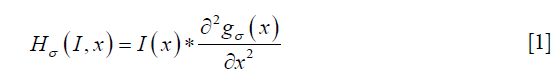
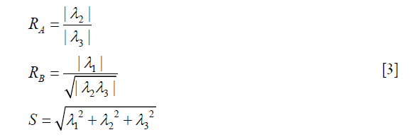
Where g_σ (x) is the Gaussian function with standard deviation σ. The local geometric information is extracted from the eigenvalues λ₁, λ₂, λ₃ of the Hessian matrix (|λ₁|≤|λ₂|≤|λ₃|). Based on the information in (38), the ideal tube structure satisfies the following requirement: (I) 0≈|λ₁|≪|λ₂|, (II) λ₂≈λ₃. Therefore, the “vesselness” at the scale σ, indicating similarity to an ideal tube structure, is calculated by the following formula,

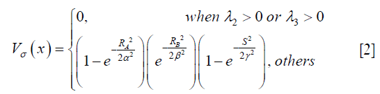
Where α, β, γ are parameters controlling sensitivity to distinguish tube-like structures, plate-like structures, blob-like structures and background, and R_A, R_B and S are

R_A, R_B and S are used to describe the dissimilarity to plate, blob and the background, respectively. After vessel enhancement, voxels representing vessels enhanced by contrast agent become brighter and other voxels become darker (Figure 5A,B).

Figure 5 Example SPGR image and feature maps: (A) SPGR image at middle time point (B) vessel-enhanced image (C) first PCA projection (D) area under curve (E) temporal standard deviation (F) SATID. These images demonstrate that voxels representing vessels (red circles) enhance on DCE-MRI and have high values on feature maps. SPGR, spoiled gradient-recalled; PCA, principal component analysis; SATID, summation of absolute temporal intensity difference.

In order to detect voxels representing the vessel compartment within cortical bone, it is necessary to identify the complete cortical region on MRI. This is more easily done using HR-pQCT data, due to better contrast between bone and soft tissue. However, distortion in the MR image causes misalignment between the HR-pQCT cortical mask and the MRI cortical region. To solve this problem, the distortion field between the HR-pQCT and the registered MRI was calculated using a modified demons registration method (39,40). In brief, the intensity of HR-pQCT was inverted and adjusted to match MRI by histogram matching, and the displacement field was acquired by applying the demons registration method to both images. This displacement field was then applied to the HR-pQCT cortical mask to create a MRI cortical bone mask. The temporal intensity of each voxel of the vessel-enhanced MRI image within the MRI cortical bone mask was extracted. Principal component analysis (PCA) was performed, and the projection of the first-component, which represents the general shape of the enhancement curve, was calculated as a feature (Figure 5C). Additionally, the area under the enhancement curve (AUC) was used as a feature because high AUC indicates contrast—and therefore vessels—exist within the voxel (Figure 5D).

While these two features identified most of the vessel-filled voxels, vessels with delayed contrast uptake time were not captured. Therefore, two more features were added to improve the detection algorithm. The first was standard deviation of temporal intensity (Figure 5E). The second was summation of absolute temporal intensity difference (SATID) (Figure 5F). SATID at point x can be calculated by the following formula,

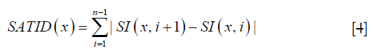
Where S1 is the temporal intensity at point x. Standard deviation and SATID will have high values in vessel-voxels due to the initial increase and subsequent decrease in signal intensity during contrast agent wash-in and wash-out.

All voxels inside the cortical bone region were clustered using a 2 stage, hierarchical k-means algorithm based on these four features (41,42). In brief, k-means clustering attempts to group all data to k clusters by iteratively minimizing the total error of each data point to its cluster center by the following formula,

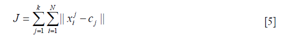
Where k is number of clusters and N is number of data points, which is number of voxels in the cortical bone region. is the data point belonging to the j-th cluster and c_j is the center of the j-th cluster. In this study, the voxels were clustered into 4 groups. The voxels belonging to the cluster with the highest average intensity and belonging to the largest five connected components were designated as “large vessels”. The remaining voxels were processed through the second stage k-means to extract smaller vessels. The final vessel mask was the union of “large vessels” and “small vessels”.

Following this process, discontinuity in the vessel mask was apparent. To repair these missing or broken vessels, a vessel connection algorithm was devised. The vessel connection algorithm performed k-means clustering with 3 groups on the full set of voxels. Those voxels belonging to the cluster with the highest average intensity were extracted, binarized, and labeled the “expanded vessel mask”. This expanded vessel mask was then skeletonized to generate an “indicator of discontinuity”. For the missing sections with indicator value “1”, the corresponding regions of the expanded vessel mask were inserted to fill in the discontinuities (Figure 6).

Figure 6 Representative result of the vessel connection algorithm. Disconnected portions of the vessel mask were detected and repaired (circles).

To quantify the proportion of vessel-filled pores in cortical bone, three quantitative metrics were used. “Vessel volume fraction” was defined as the ratio between the number of vessel voxels and cortical bone voxels,

Where V_vessel is the total number of vessel voxels and V_{cortical bone} is the total number of cortical bone voxels. “Vessel density” was defined as number of vessels per cortical bone voxel,

Where N_vessel is total count of objects in the 3D vessel map. “Average vessel volume” was defined as average number of voxels per vessel.

These metrics were calculated for both distal and ultra-distal tibia regions for each subject.

Validation

To validate the proposed vessel-filled pore detection method, and evaluate minimum detectable vessel size, a virtual phantom containing isolated, small channels of 5 different diameters (500, 400, 300, 250, 200, and 100 µm) was designed (Figure 7A). A pseudo temporal intensity for each channel was generated by imposing a baseline intensity at the first two time points and an enhanced intensity of 2× baseline at subsequent time points. The remaining voxels of the virtual phantom were assigned a low intensity representing bone tissue. A point spread function (PSF) and Gaussian noise were applied to mimic in vivo MRI data. The PSF was deconvolved (43,44) from the edge spread of intensity measured in cross sections of large, isolated channels from MRI scans of physical phantoms. The resulting virtual phantom image (Figure 7B) was processed through the image analysis pipeline to generate a vessel mask.

Figure 7 Virtual phantom with channels of varying diameter: (A) original design (B) virtual MRI data created by applying the PSF and noise derived from physical phantom scan data. MRI, magnetic resonance imaging; PSF, point spread function.

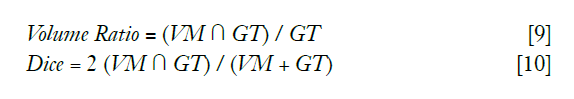
To measure the similarity between the detected vessel mask (VM) and the ground truth (GT), the overlap volume ratio and Dice coefficient of each channel was calculated by:

Results

Human subjects study

Mean vessel volume fraction was 2.2%±1.0% (2.3%±1.0% and 2.0%±1.0% at the distal and ultra-distal sites, respectively). Mean vessel density was 0.68±0.27 (0.73±0.22 and 0.63±0.31 vessel/mm³ at the distal and ultra-distal sites, respectively). Mean average vessel volume was 0.032±0.012 (0.029±0.008 and 0.035±0.014 mm³/vessel at the distal and ultra-distal sites, respectively). While no significant differences were found between the distal and ultra-distal sites (all P>0.05), mean vessel volume fraction and mean vessel density consistently trended higher at the distal site than at the ultra-distal site, while mean average vessel volume consistently trended higher at the ultra-distal site.

To confirm that the processing pipeline correctly identified vessel-filled voxels, enhancement curves for detected vessel voxels were evaluated and compared to those for voxels outside the vessel mask but within a cortical bone pore (determined based on MRI signal intensity and by comparison to HR-pQCT) (Figure 8A). Signal intensity for detected vessel voxels uniformly increased during the scan, while those for non-vessel voxels within pores did not enhance. Further, for each case, we evaluated average enhancement for all vessel voxels as compared to average enhancement for all non-vessel voxels within the cortical mask (Figures 8,9). The average intensity of detected vessel voxels increased starting at approximately 2 min, arrived the peak intensity between 5 and 7 min and maintained a high level to the end. Compared to the detected vessel voxels, the average intensity in the rest of the cortical bone was constant over the scan duration, suggesting that the proposed algorithm correctly identified vessel-filled pores from temporal DCE-MRI data (Figure 8). In the case of noisy images, the performance of the proposed algorithm was difficult to determine because for a subset of vessels true vessel enhancement was indistinguishable from noise (Figure 9).

Figure 8 Representative MRI images and graphs demonstrating the vessel detection algorithm: (A) distal tibia (B) ultra-distal tibia. Detected vessel-filled pores displayed enhancement (red box), while non-vessel filled pores did not (blue box). The mean intensity of detected vessel-filled pores (red line) also increased over the acquisition period. The mean intensity of voxels within the cortical bone boundaries excluding the detected vessel-filled pores (blue line) remained unchanged. MRI, magnetic resonance imaging.

Figure 9 Result of the vessel detection algorithm in a noisy scan (background intensity standard deviation 1,136.64). In this case, many vessel voxels were detected; however, the enhancement of a subset of detected vessel voxels was indistinguishable from noise (left).

Validation study

For channels with diameter 250 µm and larger, overlap volume ratio was 1 and dice coefficient was above 0.6. Dice coefficient exhibited a drop in value at 300 µm and did not reach 1; this was due to a vessel mask (detected volume) that was larger than the ground truth (true channel size). For channels with diameter less than 250 µm, both volume ratio and dice coefficient decreased substantially (Figure 10), suggesting that the performance of the vessel detection algorithm deteriorates when the vessel size is less than voxel size.

Figure 10 Similarity measurements comparing detected vessel voxels and ground truth for the virtual phantom.

Discussion

In this study, we developed a multi-modal image acquisition and processing pipeline to visualize and detect vasculature within cortical bone pores. In our pipeline, HR-pQCT provided the morphological information of cortical bone, and DCE-MRI provided visualization of vasculature within cortical bone. The enhancement curves of detected vessel regions suggest that the proposed vessel detection technique successfully identified vessels.

We have demonstrated that the vasculature within cortical bone can be isolated by the proposed pipeline and compared quantitative measurements between distal and ultra-distal regions of the tibia. While these results are preliminary, they demonstrate the application of the proposed algorithm in evaluating vessel status using in vivo imaging techniques. Our research program will use this technique to investigate the impact of the vascular system on pore expansion.

Based on anatomic data drawn from histological evaluations, the epi-metaphyseal arteries, which are large but few, perforate the distal tibia cortical bone through openings in both epi- and metaphyseal regions, and then branch into smaller vessels proximally (45,46). These smaller branched vessels will form a dense, interlocking vascular network proximally to connect to the branches of the nutrient vessel (47). In our quantitative metrics, we discovered: (I) average vessel size trended higher distally, and (II) mean vessel density trended higher proximally. Though it must be said that these differences did not reach statistical significance, they were consistent in all subjects. Interestingly, they are also consistent with the anatomic data, which supports fewer but larger vessels distally and more numerous but smaller vessels proximally

Using the temporal intensity variation of DCE-MRI to isolate blood vessel systems is a common strategy for vascular analysis, which assists physicians to evaluate perfusion, distinguish malignant from benign tissue, and evaluate treatment performance or disease condition. Most analysis methods include manually delineating a region of interest (ROI) and using average temporal intensity variation as an indicator (33,48,49). In the case that the enhancement curve is monotonic and smooth, several simple quantitative parameters [e.g., maximum relative enhancement (ME), time to peak (TTP)] can completely represent the curve shape. This strategy, however, needs to be modified when applied to vessel detection within cortical bone. The vessel types and sizes in cortical bone are varied, causing extreme variations of enhancement and contrast agent arrival time. Therefore, the common quantitative parameters for the voxels with vessel content vary dramatically and cause difficulty in distinguishing vessels from skeletal tissue. Temporal standard deviation and SATID, which are sensitive to temporal intensity variation, can be helpful features to detect vessels that have an unusual enhancement pattern (e.g., late TTP, small enhancement).

There are three additional differences between the proposed method and other quantitative vessel detection and analysis methods. First, most methods of quantitative vascular or perfusion analysis are applied to normalized DCE-MRI images. There are two common ways to normalize images (49-53): (I) dividing the original signal directly by the baseline signal and (II) calculating the percentage of enhancement with respect to baseline signal. In our study, however, normalization was accomplished by subtracting the baseline signal from the original signal. This was done because of the large variation in voxel intensity of cortical bone. Both standard normalization methods are sensitive to baseline intensity. For voxels with extremely low baseline intensity, normalized intensity will be high even if there is only a small intensity variation (e.g., noise): these would therefore be classified as vessel voxels. For voxels with extremely high baseline intensity, normalized intensity will be suppressed; these would be eliminated by our vessel detection algorithm. The second difference between our method and existing vessel detection methods is that existing methods attempt to extract the representative quantitative parameters directly from the normalized DCE-MRI image. In our study, we extracted parameters from the vessel-enhanced (Frangi filtered) image instead. While the temporal variation of “vesselness”—the output of Frangi filter—is highly related to intensity, the difference between vessel and background voxels will be enhanced, improving the performance of vessel detection. Third, most vessel detection methods use only a single k-means clustering to detect the desired objects. In our study, the intensity distribution of enhanced vessels has a high variance so that vessel voxels with strong features—primarily those belonging to large vessels—may dominate the k-means clustering algorithm and reduce the performance of detecting small vessels. Therefore, in a second k-means clustering step we removed voxels belonging to the largest vessels in order to increase the efficiency of small vessel detection.

The major limitation of the proposed technique is that voxel size of SPGR reconstructions is 230×230 µm² in-plane. Vessels smaller than this may not be visible, or their enhancement may be insufficient for the proposed method to classify them accurately. In our validation exam, detected volume ratio and dice coefficient decreased dramatically for channels smaller than the in-plane resolution. Conversely, if vessel size exceeds the voxel size, partial volume effects will blur the vessel objects so that voxels surrounding the vessel will also have similar temporal enhancement curves (54-57). These enhanced surrounding voxels may be incorrectly classified as vessel voxels, causing over-estimation of vessel size. In our validation exam, the Dice coefficient for vessel sizes above 250 µm decreased while the volume ratio remained equal to 1. This overestimation of vessel size can be corrected through trimming of the vessel mask with the cortical pore mask from HR-pQCT. Therefore, the proposed method does detect large vessel-filled pores, which dominate pore growth and bone biomechanics (58), enabling further research on pore expansion mechanisms. While in theory increased spatial resolution may be helpful to visualize and detect smaller vessel-filled pores, image quality will degrade and cause errors in vessel detection. Image quality would degrade with lower signal-to-noise, greater motion-induced artifacts and temporal resolution. Therefore, the current DCE-MRI protocol is a compromise between spatial resolution and image quality to optimize vessel detection.

There are additional limitations of the proposed technique that deserve discussion. First, MRI data incorporate inherent image distortion, generally small and non-critical, but which become problematic when high-resolution image processing is attempted. Even after applying the demons method to non-rigidly register MRI and HR-pQCT, the resulting MRI cortical bone mask occasionally covers voxels outside of the cortical region, leading to the occasional identification of vessel-filled pores outside of the cortical bone boundary. Second, noise on MRI images negatively influences accurate vessel detection. Temporal standard deviation and SATID are sensitive to noise. Therefore, the performance of the proposed vessel detection algorithm requires optimal MRI acquisition and reconstruction.

There are also limitations of the analysis and evaluation presented in this manuscript. First, we cannot compare to a “ground truth” of vessel-filled pore distribution for human subjects because no other in vivo technique exists to visualize and quantify them. Therefore the presented intensity curves and quantitative metrics are the only possible methods to examine the performance of the proposed processing pipeline. However, high DICE coefficient for channels larger than 250 µm demonstrate the accuracy of our processing pipeline. Second, examining the reproducibility of the proposed metrics is challenging because we are not permitted to inject contrast agent for a DCE-MRI scan more than once in the same participant due to concerns related to participant safety. Image quality and contrast uptake may vary between scans, which would influence the performance of vessel detection. However, the image analysis pipeline is completely automated and therefore fully reproducible.

UTE MRI is an alternative imaging technique to detect vessels within cortical bone. Water content in cortical bone, whether bound or free water, has extremely short relaxation time (T2*) so its signal is undetectable under conventional MRI (26,59). UTE can detect free water signal in cortical bone, located in Haversian canals (60,61). In this way, cortical porosity can be estimated from free water content mapping (25,62,63). However, the low resolution of UTE MRI hinders the visualization and spatial mapping of individual vessels.

In conclusion, we developed a multi-modal imaging and image processing technique to visualize vessel-filled pores within cortical bone. Several image processing techniques including a vessel-enhancement filter and k-means clustering were applied to enhance visualization and detection of the vessel compartment. The enhancement curves of the identified vessel voxels indicate that our algorithm can successfully detect vessel-filled pores. Future research will focus on: (I) spatially matching the vessels to cortical pores (derived from HR-pQCT image processing) for analysis of vessel proportion and distribution; (II) developing longitudinal analysis techniques to track individual pore content and growth over time, and (III) recruiting additional participants to our ongoing longitudinal study of vessel distribution and pore growth in type II diabetes.

Acknowledgments

The authors would like to acknowledge Grace Jun for her assistance with participant recruitment, Matt Tanaka for his assistance with HR-pQCT scanning, and Ravanfar Vahid and Hope Williams for their assistance with MRI scanning.

Funding: Funding support was provided by National Institutes of Health (NIH/NIAMS) grants R01AR069670, R03AR064004 and P30 DK098722 (NORC).

Footnote

Conflicts of Interest: The authors have no conflicts of interest to declare.

Ethical Statement: The UCSF Committee on Human Research approved the study protocol, and all volunteers provided written informed consent prior to participation.

References

1. Langdahl B, Ferrari S, Dempster DW. Bone modeling and remodeling: potential as therapeutic targets for the treatment of osteoporosis. Ther Adv Musculoskelet Dis 2016;8:225-35. [Crossref] [PubMed]
2. Ott SM. Cortical or Trabecular Bone: What’s the Difference? Am J Nephrol 2018;47:373-5. [Crossref] [PubMed]
3. Augat P, Schorlemmer S. The role of cortical bone and its microstructure in bone strength. Age Ageing 2006;35 Suppl 2:ii27-31. [Crossref] [PubMed]
4. Fonseca H, Moreira-Gonçalves D, Coriolano HJA, Duarte JA. Bone quality: The determinants of bone strength and fragility. Sports Med 2014;44:37-53. [Crossref] [PubMed]
5. Ohlsson C, Sundh D, Wallerek A, Nilsson M, Karlsson M, Johansson H, Mellström D, Lorentzon M. Cortical bone area predicts incident fractures independently of areal bone mineral density in older men. J Clin Endocrinol Metab 2017;102:516-24. [Crossref] [PubMed]
6. Osterhoff G, Morgan EF, Shefelbine SJ, Karim L, McNamara LM, Augat P. Bone mechanical properties and changes with osteoporosis. Injury 2016;47:S11-20. [Crossref] [PubMed]
7. Holzer G, Von Skrbensky G, Holzer LA, Pichl W. Hip fractures and the contribution of cortical versus trabecular bone to femoral neck strength. J Bone Miner Res 2009;24:468-74. [Crossref] [PubMed]
8. Poole KES, Treece GM, Mayhew PM, Vaculík J, Dungl P, Horák M, Štěpán JJ, Gee AH. Cortical thickness mapping to identify focal osteoporosis in patients with hip fracture. PLoS One 2012;7:e38466. [Crossref] [PubMed]
9. Burghardt AJ, Kazakia GJ, Ramachandran S, Link TM, Majumdar S. Age- and gender-related differences in the geometric properties and biomechanical significance of intracortical porosity in the distal radius and tibia. J Bone Miner Res 2010;25:983-93. [PubMed]
10. Nirody JA, Cheng KP, Parrish RM, Burghardt AJ, Majumdar S, Link TM, Kazakia GJ. Spatial distribution of intracortical porosity varies across age and sex. Bone 2015;75:88-95. [Crossref] [PubMed]
11. Kazakia GJ, Nirody JA, Bernstein G, Sode M, Burghardt AJ, Majumdar S. Age- and gender-related differences in cortical geometry and microstructure: Improved sensitivity by regional analysis. Bone 2013;52:623-31. [Crossref] [PubMed]
12. Patsch JM, Burghardt AJ, Yap SP, Baum T, Schwartz A V., Joseph GB, Link TM. Increased cortical porosity in type 2 diabetic postmenopausal women with fragility fractures. J Bone Miner Res 2013;28:313-24. [Crossref] [PubMed]
13. Samelson EJ, Demissie S, Cupples LA, Zhang X, Xu H, Liu CT, Boyd SK, McLean RR, Broe KE, Kiel DP, Bouxsein ML. Diabetes and Deficits in Cortical Bone Density, Microarchitecture, and Bone Size: Framingham HR-pQCT Study. J Bone Miner Res 2018;33:54-62. [Crossref] [PubMed]
14. Heilmeier U, Cheng K, Pasco C, Parrish R, Nirody J, Patsch JM, Zhang CA, Joseph GB, Burghardt AJ, Schwartz AV, Link TM, Kazakia G. Cortical bone laminar analysis reveals increased midcortical and periosteal porosity in type 2 diabetic postmenopausal women with history of fragility fractures compared to fracture-free diabetics. Osteoporos Int 2016;27:2791-802. [Crossref] [PubMed]
15. Yu EW, Putman MS, Derrico N, Abrishamanian-Garcia G, Finkelstein JS, Bouxsein ML. Defects in cortical microarchitecture among African-American women with type 2 diabetes. Osteoporos Int 2015;26:673-9. [Crossref] [PubMed]
16. Hirano T, Burr DB, Cain RL, Hock JM. Changes in geometry and cortical porosity in adult, ovary-intact rabbits after 5 months treatment with LY333334 (hPTH 1-34). Calcif Tissue Int 2000;66:456-60. [Crossref] [PubMed]
17. Lotinun S, Evans GL, Bronk JT, Bolander ME, Wronski TJ, Ritman EL, Turner RT. Continuous parathyroid hormone induces cortical porosity in the rat: Effects on bone turnover and mechanical properties. J Bone Miner Res 2004;19:1165-71. [Crossref] [PubMed]
18. Shanbhogue VV, Støving RK, Frederiksen KH, Hanson S, Brixen K, Gram J, Jørgensen NR, Hansen S. Bone structural changes after gastric bypass surgery evaluated by HR-pQCT: A two-year longitudinal study. Eur J Endocrinol 2017;176:685-93. [Crossref] [PubMed]
19. Schafer AL, Kazakia GJ, Vittinghoff E, Stewart L, Rogers SJ, Kim TY, Carter JT, Posselt AM, Pasco C, Shoback DM, Black DM. Effects of Gastric Bypass Surgery on Bone Mass and Microarchitecture Occur Early and Particularly Impact Postmenopausal Women. J Bone Miner Res 2018;33:975-86. [Crossref] [PubMed]
20. Burghardt AJ, Buie HR, Laib A, Majumdar S, Boyd SK. Reproducibility of direct quantitative measures of cortical bone microarchitecture of the distal radius and tibia by HR-pQCT. Bone 2010;47:519-28. [Crossref] [PubMed]
21. Kazakia GJ, Tjong W, Nirody JA, Burghardt AJ, Carballido-Gamio J, Patsch JM, Link T, Feeley BT, Ma CB. The influence of disuse on bone microstructure and mechanics assessed by HR-pQCT. Bone 2014;63:132-40. [Crossref] [PubMed]
22. Oei L, Koromani F, Rivadeneira F, Zillikens MC, Oei EHG. Quantitative imaging methods in osteoporosis. Quant Imaging Med Surg 2016;6:680-98. [Crossref] [PubMed]
23. Burghardt AJ, Issever AS, Schwartz A V., Davis KA, Masharani U, Majumdar S, Link TM. High-resolution peripheral quantitative computed tomographic imaging of cortical and trabecular bone microarchitecture in patients with type 2 diabetes mellitus. J Clin Endocrinol Metab 2010;95:5045-55. [Crossref] [PubMed]
24. Carey JJ, Buehring B. Current imaging techniques in osteoporosis. Clin Exp Rheumatol 2018;36 Suppl 114:115-26. [PubMed]
25. Rad HS, Lam SCB, Magland JF, Ong H, Li C, Song HK, Love J, Wehrli FW. Quantifying cortical bone water in vivo by three-dimensional ultra-short echo-time MRI. NMR Biomed 2011;24:855-64. [Crossref] [PubMed]
26. Bae WC, Chen PC, Chung CB, Masuda K, D’Lima D, Du J. Quantitative ultrashort echo time (UTE) MRI of human cortical bone: Correlation with porosity and biomechanical properties. J Bone Miner Res 2012;27:848-57. [Crossref] [PubMed]
27. Goldenstein J, Kazakia G, Majumdar S. In vivo evaluation of the presence of bone marrow in cortical porosity in postmenopausal osteopenic women. Ann Biomed Eng 2010;38:235-46. [Crossref] [PubMed]
28. Cooper DML, Turinsky AL, Sensen CW, Hallgrímsson B. Quantitative 3D analysis of the canal network in cortical bone by micro-computed tomography. Anat Rec B New Anat 2003;274:169-79. [Crossref] [PubMed]
29. Cooper DML, Thomas CDL, Clement JG, Turinsky AL, Sensen CW, Hallgrímsson B. Age-dependent change in the 3D structure of cortical porosity at the human femoral midshaft. Bone 2007;40:957-65. [Crossref] [PubMed]
30. Bousson V, Meunier A, Bergot C, Rocha MA, Morais MH. Distribution of Intracortical Porosity in Human Midfemoral Cortex by Age and Gender. J Bone Miner Res 2001;16:1308-17. [Crossref] [PubMed]
31. Chuang KH, Wu MT, Lin YR, Hsieh KS, Wu ML, Tsai SY, Ko CW, Chung HW. Application of model-free analysis in the MR assessment of pulmonary perfusion dynamics. Magn Reson Med 2005;54:299-308. [Crossref] [PubMed]
32. Agner SC, Soman S, Libfeld E, McDonald M, Rosen MA, Schnall MD, Chin D, Nosher J, Madabhushi A. Novel kinetic texture features for breast lesion classification on dynamic contrast enhanced (DCE) MRI. Proc. SPIE 6915, Medical Imaging 2008: Computer-Aided Diagnosis, 69152C.
33. You D, Aryal M, Samuels SE, Eisbruch A, Cao Y. Temporal Feature Extraction from DCE-MRI to Identify Poorly Perfused Subvolumes of Tumors Related to Outcomes of Radiation Therapy in Head and Neck Cancer. Tomography 2016;2:341-52. [Crossref] [PubMed]
34. Cuenod CA, Balvay D. Perfusion and vascular permeability: Basic concepts and measurement in DCE-CT and DCE-MRI. Diagn Interv Imaging 2013;94:1187-204. [Crossref] [PubMed]
35. Padhani AR. Dynamic contrast-enhanced MRI in clinical oncology: Current status and future directions. J Magn Reson Imaging 2002;16:407-22. [Crossref] [PubMed]
36. Liu J, Pedoia V, Heilmeier U, Ku E, Su F, Khanna S, Imboden J, Graf J, Link T, Li X. High-temporospatial-resolution dynamic contrast-enhanced (DCE) wrist MRI with variable-density pseudo-random circular Cartesian undersampling (CIRCUS) acquisition: Evaluation of perfusion in rheumatoid arthritis patients. NMR Biomed 2016;29:15-23. [Crossref] [PubMed]
37. Liu J, Saloner D. Accelerated MRI with CIRcular Cartesian UnderSampling (CIRCUS): a variable density Cartesian sampling strategy for compressed sensing and parallel imaging. Quant Imaging Med Surg 2014;4:57-67. [PubMed]
38. Frangi AF, Niessen WJ, Vincken KL, Viergever MA. Multiscale vessel enhancement filtering. In: Wells WM, Colchester A, Delp S, editors. Medical Image Computing and Computer-Assisted Intervention — MICCAI’98. MICCAI 1998. Lecture Notes in Computer Science, vol 1496. Berlin, Heidelberg: Springer, 1998. p. 130-7.
39. Thirion JP. Image matching as a diffusion process: an analogy with Maxwell’s demons. Med Image Anal 1998;2:243-60. [Crossref] [PubMed]
40. Vercauteren T, Pennec X, Perchant A, Ayache N. Diffeomorphic demons: efficient non-parametric image registration. Neuroimage 2009;45:S61-72. [Crossref] [PubMed]
41. Arthur D, Vassilvitskii S. K-Means++: the Advantages of Careful Seeding. In: Proceedings of the 18th Annual ACM-SIAM Symposium on Discrete Algorithms. 2007. p. 1027-35.
42. Lloyd S. Least-squares quantization in PCM. IEEE Trans Inf Theory 1982;28:129-37. [Crossref]
43. Jansson PA, White RL, Gilliland RL. Deconvolution of images and spectra. Deconvolution of images and spectra (2nd ed.). Academic Press; 1997. 514 p.
44. Holmes TJ, Bhattacharyya S, Cooper J, Hanzel D, Krishnamurthi V, Lin W, Roysam B, Szarowski DH, Turner JN. Light Microscopic Images Reconstructed by Maximum Likelihood Deconvolution. In: Pawley JB, editor. Handbook of biological confocal microscopy. Boston, MA: Springer US; 1995. p. 389-402.
45. Vascular anatomy of the tibia. Acta Radiol 1971;11:10-1. [Crossref]
46. Jackson RW, Macnab I. Fractures of the shaft of the tibia: A clinical and experimental study. Am J Surg 1959;97:543-57. [Crossref] [PubMed]
47. Nelson GE, Kelly PJ, Peterson LF, Janes JM. Blood supply of the human tibia. J Bone Joint Surg Am 1960;42-A:625-36. [Crossref] [PubMed]
48. Han S, Stoyanova R, Lee H, Carlin SD, Koutcher JA, Cho HJ, Ackerstaff E. Automation of pattern recognition analysis of dynamic contrast-enhanced MRI data to characterize intratumoral vascular heterogeneity. Magn Reson Med 2018;79:1736-44. [Crossref] [PubMed]
49. Khalifa F, Soliman A, El-Baz A, Abou El-Ghar M, El-Diasty T. Gimel’Farb G, Ouseph R, Dwyer AC. Models and methods for analyzing DCE-MRI: A review. Med Phys 2014;41:124301. [Crossref] [PubMed]
50. Glaßer S, Preim U, Tnnies K, Preim B. A visual analytics approach to diagnosis of breast DCE-MRI data. Comput Graph 2010;34:602-11. [Crossref]
51. Karahaliou A, Vassiou K, Arikidis NS, Skiadopoulos S, Kanavou T, Costaridou L. Assessing heterogeneity of lesion enhancement kinetics in dynamic contrast-enhanced MRI for breast cancer diagnosis. Br J Radiol 2010;83:296-309. [Crossref] [PubMed]
52. Gibbs P, Liney GP, Lowry M, Kneeshaw PJ, Turnbull LW. Differentiation of benign and malignant sub-1 cm breast lesions using dynamic contrast enhanced MRI. Breast 2004;13:115-21. [Crossref] [PubMed]
53. Arasu VA, Chen RCY, Newitt DN, Chang CB, Tso H, Hylton NM, Joe BN. Can Signal Enhancement Ratio (SER) Reduce the Number of Recommended Biopsies without Affecting Cancer Yield in Occult MRI-detected Lesions? Acad Radiol 2011;18:716-21. [Crossref] [PubMed]
54. Soret M, Bacharach SL, Buvat I. Partial-Volume Effect in PET Tumor Imaging. J Nucl Med 2007;48:932-45. [Crossref] [PubMed]
55. Rousset OG, Ma Y, Evans AC. Correction for partial volume effects in PET: Principle and Validation. J Nucl Med 1998;39:904-11. [PubMed]
56. González Ballester MA, Zisserman AP, Brady M. Estimation of the partial volume effect in MRI. Med Image Anal 2002;6:389-405. [Crossref] [PubMed]
57. Balafar MA, Ramli AR, Saripan MI, Mashohor S. Review of brain MRI image segmentation methods. Artif Intell Rev 2010;33:261-74. [Crossref]
58. Schaffler MB, Burr DB. Stiffness of compact bone: Effects of porosity and density. J Biomech 1988;21:13-6. [Crossref] [PubMed]
59. Reichert IL, Robson MD, Gatehouse PD, He T, Chappell KE, Holmes J, Girgis S, Bydder GM. Magnetic resonance imaging of cortical bone with ultrashort TE pulse sequences. Magn Reson Imaging 2005;23:611-8. [Crossref] [PubMed]
60. Wehrli FW, Song HK, Saha PK, Wright AC. Quantitative MRI for the assessment of bone structure and function. NMR Biomed 2006;19:731-64. [Crossref] [PubMed]
61. Yeni YN, Brown C, Norman T. Influence of Bone Composition and Apparent Density on Fracture Toughness of the Human Femur and Tibia. Bone 1998;22:79-84. [Crossref] [PubMed]
62. Bae WC, Patil S, Biswas R, Li S, Chang EY, Statum S, D'Lima DD, Chung CB, Du J. Magnetic resonance imaging assessed cortical porosity is highly correlated with µCT porosity. Bone 2014;66:56-61. [Crossref] [PubMed]
63. Techawiboonwong A, Song HK, Leonard MB, Wehrli FW. Cortical Bone Water: In Vivo Quantification with Ultrashort Echo-Time MR Imaging. Radiology. 2008;248:824-33. [Crossref] [PubMed]