

Shading correction for volumetric CT using deep convolutional neural network and adaptive filter
Introduction
Volumetric CT (VCT) is widely used in image-guided radiation therapy. Due to scatter and beam hardening in VCT scanning, a low-frequency shading artifact severely deteriorates the quality of the reconstructed image. Shading artifact causes reconstructed image inaccuracy and spatial non-uniformity (SNU). Without shading correction, the CT number error of reconstructed image CT will be exceeded 350 HU, which brings errors to the positioning accuracy of image-guided treatment and the diagnosis of the image. Thus, it limits the VCT in the clinical application. Therefore, shading correction in VCT is one of the most important problems to be solved for improving VCT image quality.
The importance of shading correction on the VCT system is reported by many publications on this topic (1-12). The existing methods of shading correction are mainly divided into two types: pre-processing and post-processing. The pre-processing method corrects the shading artifact in VCT image mainly using an additional hardware device, aiming to prevent the scattering photon from reaching the detector. Following are two typical methods for shading correction in pre-processing. The first one is increasing the air gap between object and detector (13). As the air gap widens, the detection efficiency of the scattered photons will be reduced because of the small cone angle. However, this method is limited by the physical space of the VCT system because the spatial distance cannot be increased indefinitely.
Meanwhile, the X-ray dose will be increased to compensate for the enlarged distance, which is not practical in the clinic. The second one is using the anti-scatter grid (14), which can block the scattered signal of incident angle, while the attenuation efficiency of scattered light using this method is not high enough. At present, the commercial grid can only provide about three times reduction rate of the scatter-primary ratio (SPR), which cannot guarantee the quality of VCT image in a high scattering environment. It also needs to increase the radiation dose to compensate for the attenuation of the X-ray intensity.
Although pre-processing can directly prevent the scattering photon from reaching the detector, its limitation is obvious, and post-processing is more practical. Post-processing methods include analytical modeling (15), Monte Carlo simulation (16,17), modulation method (3), measurement-based method (1-3,6,18), and scatter correction based on prior data (19,20). Analytical modeling method has a fast computation speed, but the accuracy of scattering estimation is not high enough especially in the complex object. Monte Carlo simulation is the “golden standard” for scattering estimation, but the method is time-consuming. Modulation method adds a high-frequency modulator between kV X-ray tube and the scanned object. According to different response characteristics between primary and scatter signal, they could be separated in the frequency domain. However, the modulator must be static in the projection, which requires a high accuracy geometry VCT system. Due to the gantry rotation wobble, its clinical application is limited. The measurement-based method requires inserted blocker (usually using lead) into the X-ray source and scanned object (1-3,6,21-25). In this way, the detector forms the shadow region that only contains the scatter signal, but such a methodology is difficult to operate by changing the hardware setting of the existing system. Shading correction based on prior data can get the corrected image better, but this method needs additional prior patient information. Therefore, it cannot be used as a general solution for shading correction.
To tackle the issues in shading correction, in this paper, a novel approach is proposed incorporating the deep convolutional neural network (DCNN) and adaptive filter (AF) together to estimate the shading artifact accurately, which fully explore the potential of DCNN in segmentation of the VCT image with severe artifact and extract the shading artifact using AF (26). The proposed method does not depend on the prior image data and is completely compatible with the linear accelerator in image-guided radiotherapy (IGRT). It does not need to change other hardware and scan protocols and simultaneously without increasing scanning time and dose.
Methods
Workflow
As is known, CT numbers of the same human tissues are approximately the same (26). According to this feature, a template image without shading artifact can be constructed by image segmentation and be used as the corrected reference. To isolate the shading artifacts from the raw data, we generate the residual image by subtracting template image from raw data. An AF is applied in the residual image to estimate the shading artifact so that we can extract the shading artifact while maintaining structure and detail.
Figure 1 shows the framework of the shading artifact correction using DCNNAF. Due to the image SNU effect by shading artifact, the conventional segmentation algorithm is difficult to distinguish the different human tissues. We propose a DCNN to extract deep feature about the VCT image with shading artifact so that an accurate segmentation can be achieved to distinguish the different tissues. Before we start the framework, the input VCT images Itrain and the corresponding labels of segmentation Ilabel are applied to train DCNN. To start the framework, we input the reconstructed VCT images I0 with shading artifacts to the trained DCNN. The template image It is generated from the output of the DCNN. The residual image Ir which is generated by the subtracting segmented image from the uncorrected image has shading artifact, structure and image detail. The structure and image detail is the high-frequency signal while the shading artifact is the low-frequency signal. Therefore, an AF is implemented to the residual image to remove the high-frequency signal. The shading artifact at low frequency can be obtained. Finally, the artifact is compensated for the raw image to get the final image. The following sections introduce the key steps in the workflow, including VCT segmentation using DCNN and shading artifact estimation using an AF.

VCT segmentation using DCNN
Dramatic developments in parallel technology enable the processing of big data for DCNN. Semantic pixel-wise segmentation is an ongoing topic of research, which is improved by deep learning. Unlike the existing conventional segmentation algorithm, segmentation using DCNN is not just based on the image intensity, so that it is especially suitable for shading contaminated VCT image segmentation. This paper proposes a deep convolutional encoder-decoder architecture for robust and accurate human tissue segmentation (bone, marrow, muscle, fat, and air), which can generate an accurate template image assisting shading correction.
DCNN architecture
The black dotted box in Figure 1 demonstrates the DCNN. The encoding part and the decoding part are shown in the left and right side (27), respectively. The encoding part follows the convolutional neural network, and the repeated convolution layers are included. The Rectified Linear Unit (ReLU) layer follows the convolution layer. In the down-sampling step, the max pooling operation with the size of 2×2 and the stride of 2 is applied. The number of feature channels is doubled at each down-sampling step. In the decoding part, a concatenation layer from the correspondingly down-sampling step (shown in the gray arrow in Figure 1) is copied to the step of up-sampling. The up-sampling convolutional layer with 2×2 filter kernel contains the half number of feature channels. Therefore, the output image can be resized into the same size as the input image. The 3×3 convolutions with ReLU are followed by the max pooling and up-convolution layers. In the final step, a 1×1 convolution layer and a soft-max layer are proposed to map the target of segmented tissue. The proposed DCNN architecture of tissue segmentation has 24 convolutional layers.
Network training
The DCNN architecture aims to obtain the mapping function between the input image and the output of the segmented image. To train the DCNN is to improve the accurate of pixel classification from the VCT image. The final segmentation output from the DCNN can be written as:
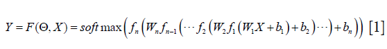
Where X is the input of VCT raw data, Y is the image label with the segmented tissue, bi is the bias in the ith convolution layer, Wi is the ith convolution layer, fi is a ReLU function in ith convolution layer, Θ represents all the tuning parameters in the training step. softmax is the classification layer, which is widely used in image segmentation. The aim of the DCNN architecture is to figure out a set of optimal parameters Θ with the input of the image to minimize the loss function:
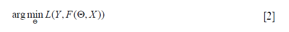
In this equation, L represents the loss of cross-entropy in segmentation. Since the loss function and the ReLU are differentiable, the back-propagation algorithm can be applied to minimize Eq. [2]. In this study, the DCNN was trained using the Adam algorithm. The learning rate was initially set at 10−3 and the factor for dropping the learning rate is 0.1 in the ten epochs passes. The size of the mini-batch was 16. DCNN is implemented using Matlab R2018a on a graphics workstation. It has an Intel Core Xeon E5-2697 v3 CPU and 128 GB RAM. Two GPU cards (Nvidia GTX Titan Xp) are used to accelerate the minimization step of the loss function. The tuning parameters Θ are initialized with a random number between −1 and 1.
Training datasets
In this study, the proposed DCNN architecture is applied to the two datasets for testing the practicability of tissue segmentation. The two datasets are introduced as follows:
- Catphan©504 phantom dataset. We have collected ten subjects of the projections with different current and voltage of the X-ray tube. The VCT projections were acquired with tabletop VCT systems. The ten subjects of VCT projections were reconstructed using FDK reconstruction algorithm. The reconstructed voxel is 512×512×200. The voxel size of the image is 0.5×0.5×0.5 mm3. A total of 2,000 two-dimensional (2D) VCT images were obtained.
- Patient pelvis image dataset. The patient’s VCT data are collected on the On-Board Imager (OBI) which is equipped on Varian Trilogy. The pelvis dataset consists of 15 subjects with a different patient. The reconstructed voxel is 512×512×56. The voxel size of the image is 0.98×0.98×2.5 mm3. A total of 840 2D VCT images were obtained.
The VCT images in both datasets are aligned to the corresponding label with the different segmentation targets. In the phantom dataset, Teflon, Delrin, Acrylic, Low-Density Polystyrene, water, polymethylpentene, and air are contoured as the target of segmentation. In the patient pelvis image dataset, we segment the image into the air, fat, muscle, marrow and bone. Two networks are trained for the phantom and patient pelvis, respectively. To verify the DCNN network, we divided the VCT image datasets into three categories: training dataset, the validation dataset, and the testing dataset. The training dataset is 80% of the VCT images, while the validation dataset is 20% of the VCT images. The testing dataset is 200 slice of the phantom image and 56 slices of patient pelvis image. The images in these three datasets are different.
Shading artifact estimation using an AF
The segmentation image is obtained from the output of the DCNN. The corresponding tissue area is filled with the standard CT number of corresponding X-ray tube voltage, to generate a template image It, and this image has no image details. By subtracting the raw images from the template image It, the residual image R is generated. The residual image contains the shading artifact and the image detail. The shading artifacts are mainly low-frequency signals while the image details are mainly high-frequency signals. Therefore, a low pass filter can be used to separate the shading artifact and image details. Conventional low pass filter can eliminate the image detail, but the boundary of the anatomical structure in the residual image R may be filtered out simultaneously, resulting in the severe loss of image contrast. Consequently, the filter should balance image smoothing and edge preserving. In this paper, a L0 norm smoothing filter is applied to the residual image which can achieve smoothing the image detail while preserving the edge of the structure. The objective function of the filter is as follow:
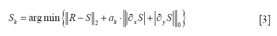
Here S is the estimated shading artifact, R is the residual image. ∂xS and ∂yS are the gradient of shading artifact in x and y direction, respectively. ak is a weight directly controlling the degree of smoothing. ║R−S║2 is a constraint of the image structure similarity. A discrete counting metric is applied in the objective function. Since the first term is the pixel-wise difference while the second term is global discontinuity statistically, discrete and the traditional gradient optimization methods are incapable of solving this problem. We apply a special alternating optimization strategy with half-quadratic splitting to solve the objective function (28).
The smoothing image Sk is significantly depended on the smoothing parameter ak. In this paper, we propose an adaptive framework to choose a suitable ak automatically, which can achieve the shading correction and image structure protection. Since the shading artifact deteriorates the spatial uniformity of the image, the goal of shading correction is to improve the spatial uniformity in the same tissue. To find a correct smoothing parameter ak, we figure out the solution based on the assumption that CT numbers of the same human tissues are approximately the same. From the above assumption, we can know that the ideal CT image has high spatial uniformity in the specific tissue. In this paper, we use a sharp peak in the image histogram of the specific tissue to represent the spatial uniformity of the image. Therefore, a suitable value of the smoothing parameter ak is calculated as an optimization model to minimize the objective function. The function is written as follows:
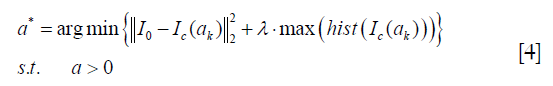
Where I0 is the input of the uncorrected image, Ic(ak) is the output of the corrected image with the smoothing parameter setting at ak. hist is the image histogram in the specific tissue.  is the image fidelity term, which can protect the structure of the output image. is the term of image spatial uniformity. λ is a penalty factor which is set at −10−3 empirically.
Eq. [4] is solved using the mesh adaptive direct search (MADS) algorithm. The convergence analysis for the MADS algorithm can be found in Ref. (29). It can achieve automatic smoothing parameter setting instead of cockamamie tuning. After getting a suitable parameter of the filter, the final corrected image can be obtained using the following formula:
Where S* is the estimated shading artifact with smoothing parameter setting at a*.
Pseudocode
In summary, we present the pseudo-code using the DCNNAF algorithm for the shading correction in Table 1. Line 1 sets the DCNN architecture and the training parameters. Line 2 gives the optimization control parameters, including the stopping criteria and initial setting. Line 3 is the training step to minimize the cross-entropy using Adam algorithm. Line 4 is the predicting step that is using the trained network to segment the input image. Line 5 is the generation step of the residual image. Line 6–23 is the main loop of generating the AF. In the step of the AF, Line 7 is the smoothing step on the residual image in order to estimate the shading artifact. Line 8 indicates the generation of the temporary corrected image. Lines 9–11 apply a barrier function ψ(ak) to change the constraint optimization problem into an unconstraint optimization problem. The barrier objective function G(ak) is solved using MADS algorithm shown in line 12–23. The searching step in Lines 12–15 is implemented to find a new iteration that decreases the objective function in Mk. When the step of searching fails to find the decreased value, the polling step in Lines 16–20 is performed in the current iteration. When the step of polling also fails to find the decreased value, the parameter of mesh-size is decreased. Otherwise, the parameter of mesh-size is increased. To terminate the iterative process, the stopping criteria Δtol should be smaller than a given threshold after a certain number of iterations (kmax) in Lines 21–23. Lines 24–25 are implemented to compensate the estimated shading artifact into the uncorrected image to get the final image.

Full table
Evaluation
The DCNNAD method is evaluated using the Catphan©504 phantom and patient pelvis cases. The phantom projection is acquired using the tabletop VCT system at Shenzhen Institutes of Advanced Technology, Chinese Academy of Sciences. The geometry of the tabletop VCT system matches with the Varian Trilogy OBI. We also obtained the phantom image using the narrow collimation in front of the kV tube (a width of around 10 mm on the detector). In this fan beam equivalent geometry, scatter signals are inherently suppressed, and the resultant images were referred to as “scatter-free” reference images for comparison. After the Catphan©504 phantom study, the pelvis image of the patient is included to evaluate the practicability and robustness of the proposed DCNNAF algorithm. The pelvis data sets are acquired from patients on Varian Trilogy OBI at the Department of Radiation Oncology. For comparison, the corresponding planning CT of a patient is also acquired as the reference image.
Table 2 lists the scanning and reconstruction parameters. We apply the image contrast and SNU as quality metrics in the regions of interest (ROIs) of the image. Scatter artifacts are more prominent around objects with high contrasts. On Catphan©504 phantom study, the image contrast was calculated as:

Full table
Where μr is the mean CT number of VCT image inside ROI and μb is the mean CT number of VCT image in the surrounding area. Since the scatter signals cause non-uniformity in the VCT image, the SNU (30) is measured as:
Where  and are the maximum and the minimum of the mean CT numbers the selected ROIs, respectively. Five ROIs with the same diameter of 10 pixels (5.0 mm) were selected in the VCT image of the Catphan©504 and patient pelvis data.
Results
Catphan©504 studies
Figure 2 shows the effects of the scatter correction using the proposed scheme on the reconstructed VCT images. Due to the scatter signal in the projection, the reconstruction error is significant as shown in Figure 2A and D. Since the shading correction is implemented using the DCNNAF method, the shading artifacts are suppressed as demonstrated in Figure 2B and E. Figure 2C and F shows the referenced fan-beam CT image. The average CT numbers in the selected ROIs from Figure 2A,B,C are −40, 58 and 69 HU, respectively. Consequently, the average absolute error of CT numbers is 109 and 11 HU in the uncorrected and corrected image, respectively. It demonstrates the significant improvement of the proposed method. We evaluated the spatial resolution using the modulation transfer function (MTF). A circular object (the red box in Figure 2) is selected for MTF calculation. The 50% of MTF magnitude is 4.77 in the corrected image while the 50% of MTF magnitude is 4.56 in the uncorrected image. After correcting the scatter, the spatial resolution in the corrected image is higher than the uncorrected image. The 1D profiles of the CT number along with the dashed white line passing through the two high-contrast rods in Figure 2B is shown in Figure 3. The 1D profiles match well with the reference image using the proposed method.


For further evaluation of the scatter correction performance using the proposed scheme, the average CT numbers and contrasts are calculated for the contrast rods in one of the phantom inserts as indicated in Figure 2A. The results are summarized in Table 3 using a fan-beam CT as the reference. The CT number error is reduced from 206 to 13 HU in the selected ROI with the implementation of the proposed method. The image contrast is increased by a factor of 1.46 on average.

Full table
Since the Catphan©504 is of the regular structure with an almost uniform distribution of CT number, a more challenge evaluation will be presented in the heterogeneous pelvis patient study in the next section.
Patient head studies
For more challenging, a patient pelvis image obtained on the clinical VCT is evaluated using the proposed framework. Figure 4 shows the result of the processing image using DCNNAF; the 1–3th row is the axial, coronal and sagittal view image, respectively. The shading artifact severely deteriorates the image as shown in Figure 4A,E,I, leading to spatial non-uniformity in the pelvis image. Figure 4B,F,J shows the segmentation image. Although the shading artifact poses a big challenge in the segmentation of different tissue, the proposed DCNN method can achieve high accurate segmentation in bone, marrow, muscle, fat, and air mainly due to the deep feature extraction in the training data. Accurate segmentation makes the directly shading correction in image-domain a possible. Figure 4C,G,K shows the corrected image, which is significantly suppressed the shading artifact presented in the raw images. The corrected image using DCNNAF method is comparable to the registered planning CT is shown in Figure 4D,H,L. For quantitative image quality analysis, the error of CT number is reduced from 198 to 10 HU in the soft tissue region enclosed by the solid red circle in Figure 4A. The SNU is calculated in the five selected ROIs which are shown in Figure 4A. The SNU in the uncorrected and corrected image is reduced from 24% to 9%.

Discussion
In this work, we investigated the DCNN in the segmentation of VCT image with severe shading artifact and proposed an AF to correct the shading artifact. Contrasted with the conventional shading correction method (31), the proposed DCNNAF method not only achieves high-quality image but also has a high computational efficiency due to the image-domain processing. Though we have tackled several issues in shading correction, the proposed scheme can be further improved. First, although the prediction is high computational efficiency, the proposed DCNN architecture spends a long time for data training, which generally takes one day to get a trained model, while the traditional segmentation does not need to train. In the future, we will improve the computational efficiency of data training by reducing the capacity of the network with high accuracy of segmentation. Second, the DCNN architecture needs large numbers of training data, and the corresponding labels of segmentation are needed to be contoured manually. The example of training data and corresponding label are shown in Figure 5A and B. In Figure 5B, it is evident that the label image which is contoured manually has a sharp edge between the different tissues. The error of the contoured image is unavoidable. Even so, the prediction of the testing image has a highly accurate result of segmentation, and the sharp edge error is eliminated shown in Figure 5C and D. It demonstrates that the DCNN can tolerate contoured error.

Different parameters will influence the accuracy of segmentation. The filter size of the convolutional layer needs to be optimized. We determine the optimized value by changing the filter size while keeping the other parameter fixed. Figure 6 shows the influence of the filter size on the patient dataset. As compared with the filter size of 1, 5, and 7, the proposed filter size 3 achieve higher accuracy at the last epoch. Therefore, we choose 3 as the best filter size.

Currently, we apply the DCNNAF method to only focus on patient pelvis data. We will extend the study on all parts of human VCT image. Regarding the patient pelvis, we focus on four tissues, i.e., bone, marrow, muscle, and fat in this paper. More tissue classification needs to be done in the future to improve the robustness of the proposed method around the whole part of the human VCT images, as well as its practicability to clinical application. Unsupervised learning is developing fast (32), and it also can achieve segmentation method. In this study, the proposed workflow still requires a large amount of training data and segmentation labels. In the future, our team would do more searches on unsupervised learning that needs less training data on this problem.
Conclusions
In this study, we propose a robust shading correction method using DCNNAF, which improves the VCT image quality. It does not need to change other hardware and scan protocols. The method also does not increase the scanning time, and the deliver X-ray dose. On the Catphan©504 study, the error of the CT number in the corrected image’s ROI is reduced from 109 to 11 HU. On the patient pelvis study, the error of the CT number in the selected ROI is reduced from 198 to 10 HU. Besides the high shading correction efficacy, the proposed method possesses several advantages over other existing shading correction approaches, including no dose or extra scan time, no requirement of prior knowledge, easy implementations and high quality of the corrected images.
Acknowledgments
The authors would like to thank the anonymous reviewers for their constructive suggestions which substantially strengthen the paper.
Funding: This work is supported in part by grants from the National Key Research and Develop Program of China (2016YFC0105102), the Leading Talent of Special Support Project in Guangdong (2016TX03R139), Fundamental Research Program of Shenzhen (JCYJ20170413162458312), the Science Foundation of Guangdong (2017B020229002, 2015B020233011, 2014A030312006) and CAS Key Laboratory of Human-Machine Intelligence-Synergy Systems, Shenzhen Institutes of Advanced Technology, and the National Natural Science Foundation of China (61871374, 81871433).
Footnote
Conflicts of Interest: The authors have no conflicts of interest to declare.
References
- Min J, Pua R, Kim I, Han B, Cho S. Analytic image reconstruction from partial data for a single-scan cone-beam CT with scatter correction. Med Phys 2015;42:6625-40. [Crossref] [PubMed]
- Niu T, Zhu L. Scatter correction for full-fan volumetric CT using a stationary beam blocker in a single full scan. Med Phys 2011;38:6027-38. [Crossref] [PubMed]
- Zhu L, Bennett NR, Fahrig R. Scatter correction method for X-ray CT using primary modulation: theory and preliminary results. IEEE Trans Med Imaging 2006;25:1573-87. [Crossref] [PubMed]
- Zhang Z, Liang X, Dong X, Xie Y, Cao G. A Sparse-View CT Reconstruction Method Based on Combination of DenseNet and Deconvolution. IEEE Trans Med Imaging 2018;37:1407-17. [Crossref] [PubMed]
- Li H, Mohan R, Zhu XR. Scatter kernel estimation with an edge-spread function method for cone-beam computed tomography imaging. Phys Med Biol 2008;53:6729-48. [Crossref] [PubMed]
- Lee H, Xing L, Lee R, Fahimian BP. Scatter correction in cone-beam CT via a half beam blocker technique allowing simultaneous acquisition of scatter and image information. Med Phys 2012;39:2386-95. [Crossref] [PubMed]
- Zhao W, Vernekohl D, Zhu J, Wang L, Xing L. A model-based scatter artifacts correction for cone beam CT. Med Phys 2016;43:1736. [Crossref] [PubMed]
- Shi L, Vedantham S, Karellas A, Zhu LJ. X-ray scatter correction for dedicated cone beam breast CT using a forward-projection model. Med Phys 2017;44:2312-20. [Crossref] [PubMed]
- Yang C, Wu P, Gong S, Wang J, Lyu Q, Tang X, Niu TJ. Shading correction assisted iterative cone-beam CT reconstruction. Phys Med Biol 2017;62:8495-520. [Crossref] [PubMed]
- Zhao C, Zhong Y, Wang J, Jin M. editors. Simultaneous Dose Reduction and Scatter Correction for 4D Cone-Beam Computed Tomography. 2017 IEEE Nuclear Science Symposium and Medical Imaging Conference (NSS/MIC); 2017: IEEE. Available online: https://doi.org/ [Crossref]
- Liang X, Zhang Z, Niu T, Yu S, Wu S, Li Z, Zhang H, Xie Y. Iterative image-domain ring artifact removal in cone-beam CT. Phys Med Biol 2017;62:5276-92. [Crossref] [PubMed]
- Shi L, Vedantham S, Karellas A, Zhu L. The role of off focus radiation in scatter correction for dedicated cone beam breast CT. Med Phys 2018;45:191-201. [Crossref] [PubMed]
- Cai W, Ning R, Conover D. Scatter correction using beam stop array algorithm for cone-beam CT breast imaging. Medical Imaging, 2006.
- Siewerdsen JH, Moseley DJ, Bakhtiar B, Richard S, Jaffray DA. The influence of antiscatter grids on soft-tissue detectability in cone-beam computed tomography with flat-panel detectors. Med Phys 2004;31:3506-20. [Crossref] [PubMed]
- Spies L, Evans PM, Partridge M, Hansen VN, Bortfeld T. Direct measurement and analytical modeling of scatter in portal imaging. Med Phys 2000;27:462-71. [Crossref] [PubMed]
- Xu Y, Bai T, Yan H, Ouyang L, Pompos A, Wang J, Zhou L, Jiang SB, Jia X. A practical cone-beam CT scatter correction method with optimized Monte Carlo simulations for image-guided radiation therapy. Phys Med Biol 2015;60:3567-87. [Crossref] [PubMed]
- Zbijewski W, Beekman FJ. Efficient Monte Carlo based scatter artifact reduction in cone-beam micro-CT. IEEE Trans Med Imaging 2006;25:817-27. [Crossref] [PubMed]
- Wang J, Solberg T. Scatter Correction for Cone-beam Computed Tomography Using Moving Blocker. Med Phys 2010;37:5792. [Crossref] [PubMed]
- Niu T, Sun M, Star-Lack J, Gao H, Fan Q, Lei Z. Shading correction for on-board cone-beam CT in radiation therapy using planning MDCT images. Med Phys 2010;37:5395-406. [Crossref] [PubMed]
- Liang X, Jiang Y, Niu T. Quantitative cone-beam CT imaging in radiotherapy: Parallel computation and comprehensive evaluation on the TrueBeam system. IEEE Access 2019.
- Liu X, Shaw CC, Wang T, Chen L, Altunbas MC, Kappadath SC. An accurate scatter measurement and correction technique for cone beam breast CT imaging using scanning sampled measurement (SSM) technique. Proc SPIE Int Soc Opt Eng 2006;6142:6142341-7.
- Zhu L, Xie Y, Wang J, Xing L. Scatter correction for cone-beam CT in radiation therapy. Med Phys 2009;36:2258-68. [Crossref] [PubMed]
- Yan H, Mou X, Tang S, Xu Q, Zankl M. Projection correlation based view interpolation for cone beam CT: primary fluence restoration in scatter measurement with a moving beam stop array. Phys Med Biol 2010;55:6353-75. [Crossref] [PubMed]
- Liang X, Gong S, Zhou Q, Zhang Z, Xie Y, Niu T. SU-F-J-211: Scatter Correction for Clinical Cone-Beam CT System Using An Optimized Stationary Beam Blocker with a Single Scan. Med Phys 2016;43:3457. [Crossref]
- Zhao C, Zhong Y, Duan X, Zhang Y, Huang X, Wang J, Jin M. 4D cone-beam computed tomography (CBCT) using a moving blocker for simultaneous radiation dose reduction and scatter correction. Phys Med Biol 2018;63:115007. [Crossref] [PubMed]
- Wu P, Sun X, Hu H, Mao T, Zhao W, Sheng K, Cheung AA, Niu T. Iterative CT shading correction with no prior information. Phys Med Biol 2015;60:8437-55. [Crossref] [PubMed]
- Ronneberger O, Fischer P, Brox T. U-Net: Convolutional Networks for Biomedical Image Segmentation. International Conference on Medical Image Computing and Computer-Assisted Intervention, 2015.
- Xu L, Lu C, Xu Y, Jia J. Image smoothing via L0 gradient minimization. ACM Trans Graph 2011;30:174. [Crossref]
- Audet C, Dennis JE Jr. Mesh Adaptive Direct Search Algorithms for Constrained Optimization. Siam Journal on Optimization 2004;17:188-217. [Crossref]
- Shi L, Vedantham S, Karellas A, Zhu L. Library based x-ray scatter correction for dedicated cone beam breast CT. Med Phys 2016;43:4529. [Crossref] [PubMed]
- Fan Q, Lu B, Park JC, Niu T, Li JG, Liu C, Zhu L. Image-domain shading correction for cone-beam CT without prior patient information. J Appl Clin Med Phys 2015;16:65-75. [Crossref] [PubMed]
- Kallenberg M, Petersen K, Nielsen M, Ng A, Diao P, Igel C, Vachon C, Holland K, Karssemeijer N, Lillholm M. Unsupervised deep learning applied to breast density segmentation and mammographic risk scoring. IEEE Trans Med Imaging 2016;35:1322-31. [Crossref] [PubMed]

