
Uniform enhancement of optical micro-angiography images using Rayleigh contrast-limited adaptive histogram equalization
Introduction
Label-free optical hemodynamic imaging has made possible the visualization of moving red blood cells inside vessels and separating them from surrounding tissues (1). Such complementary information to the tissue microstructure can be used to monitor physiological and pathological behaviors of living tissue (2). Developmental tissues such as regeneration and maturation, is always accompanied by formation of new vessels (angiogenesis), and monitoring of this progress can be useful in numerous research and clinical applications (3). Also, some diseases are directly or indirectly related to or influenced by the functional microvasculature, for example stroke and traumatic brain injury (4), diabetes (5), wound healing (6), glaucoma (7) and age-related macular degeneration (8).
Optical micro-angiography (OMAG) is a label-free non-invasive imaging and processing method to obtain three-dimensional blood perfusion map in microcirculatory tissue beds in vivo using Fourier-domain optical coherence tomography (FD-OCT) (1). Since it was reported in 2007, it has been advanced to have a sensitivity of 4 µm/s, sufficient to image the blood flow within capillary vessels (9). To obtain 3D map of the microvasculatural tissue bed, there are a number of data processing methods proposed, which include Hilbert transformation to separate the blood flow signals from the static tissue background signals in one step (10,11), simple high-pass filtering approach to extract the blood flow signals from the output OCT signals (9,12,13), and more recently the eigendecomposition- (ED-) based OMAG algorithm that was based on the eigen decomposition of the FD-OCT signals to separate static structure tissue and dynamic scatters (red blood cells) (14). OMAG has been applied to visualize blood perfusion and micro-vasculature map in various tissue samples such as retina (15), brain (16), renal microcirculation (17) and skin (13).
When the imaging is performed, the probing light is subject to specular reflection at the tissue surface when it shines onto tissue. Furthermore, the propagation of light within the tissue suffers from attenuation and scattering which makes the backscattering light collected at the detector non-uniform. These physical limitations can result in local imaging contrast degraded, leading to non-uniform appearance of the micro-angiogram images. This situation is more serious when a large area of the tissue is imaged, in which because of the limited field of view of the current scanning mechanism of the probe beam, multiple tile images are needed to acquire and stitch together (mosaicking) to form a final image. In such circumstance, even by fixing the visualization dynamic range for each of the image tiles, yet, the final vasculature map will not be homogeneous throughout the entire image.
Figure 1A shows the vasculature map in mouse ear which is formed by stitching 22 OMAG images together. Although the dynamic range in all of the images is identical, an obvious difference is observed between their background and contrast. It can be observed that the background on the lower part of the ear is relatively higher than the other areas. Also, some small vessels and capillary loops on the ear edge are with very low contrast. Similarly, Figure 1B shows the vasculature map in another mouse ear, which is the result of stitching 29 OMAG images together. The background inhomogeneity due to specular reflection and low signal at capillary loops is significant, affecting the visualization and eventual quantification. Also, the intensity value at some large vessels is saturated. Due to these problems, OMAG images acquired at different time points or from different animals would not be repeatable, especially when quantifying some vessel parameters such as vessel area density and vessel diameter are required.

In order to solve this problem, a post-processing step is required. Digital contrast enhancement is a post-processing technique applied to digital images to qualitatively improve the contrast of images. This process allows fixed or adaptive manipulation of the dynamic range such that the results are more informative for human eye. Normal human visual system can only distinguish less than ~100 different gray levels. However, current technology allows for capturing digital images at very higher bit information (12-14 bits or higher) which is about a few thousand levels. In order to distinguish an object from its surrounding environment, a good contrast in the image is required. Contrast is defined as the difference in luminance between the object of interest and the other objects at the same field of view. The post-processing algorithms are popular in the field of radiology (18), computed tomography (19) and digital mammography (20) where the contrast of the images are typically low and requires manual/automatic enhancement for better diagnosis.
In other words, the goal of this post-processing step is to map a given intensity value of one specific pixel (and its surroundings) of the input image, to an output value to form a visually uniform, informative and high-contrast image in the output. The existing contrast enhancing and normalization algorithms can be divided into two categories: static and adaptive. In static algorithms such as intensity windowing, a small range of input intensity dynamic range is stretched to the entire visualization dynamic range and the values below and above the limits are saturated. Histogram of an image is the probability distribution function (PDF) of the occurrence of one specific gray level in that image. Histogram equalization (HE) is a contrast enhancement technique that increases the global contrast of images when the information content is represented by close contrast values. HE method maps input intensities to an output image where its PDF is uniform and its cumulative distribution function (CDF) histogram is the same as the input image. This allows stretching the contrast of the image to be distributed uniformly in the dynamic range (21). However, HE may produce unrealistic images and amplify background noise while decreasing the usable data. HE has been generalized to local histogram equalization which divides the input image into smaller regions and applies HE algorithm to create a uniform distribution in each region. This method is commonly known as adaptive histogram equalization (AHE) (22). One of the disadvantages of AHE is noise amplification in homogenous regions. In order to overcome this limitation, contrast limited adaptive histogram equalization (CLAHE) was proposed (23,24). CLAHE limits amplification of noise by clipping the histogram at a pre-defined value before computing the CDF that limits the slope of the output CDF and eventually the transformation function. High peaks in the histograms are usually caused by uniform regions. The advantage of CLAHE is that it equally redistributes the part of the histogram above a clip limit among all histogram bins. Yet, a uniform PDF distribution is not ideal because it would simultaneously distribute the dynamic range between background and foreground and also amplify the noise effect. In order to improve the contrast of OMAG images while not saturating uniform and high intensity areas, non-uniform distribution functions such as Rayleigh (bell shape) distribution can be used. Intuitively, the Rayleigh distribution of OMAG image imposes this condition in that intensities are distributed evenly between small and large vessels, larger vessels are not saturated and there is a good contrast between vessels and their background. Although some other distributions such as Gaussian and exponential can be used instead, we have experimentally observed better results with Rayleigh distribution.
In this paper, we propose using Rayleigh contrast-limited adaptive histogram equalization (RCLAHE) technique to create a high-contrast and visually more homogenous OMAG images and a good background/foreground separation without changing physical OMAG quantitative parameters such as vessel area density, vessel length fraction and fractal dimension (25). We also compare the results with some existing methods from the qualitative and quantitative point of view.
Methodology
Rayleigh contrast-limited adaptive histogram equalization (RCLAHE)
The RCLAHE algorithm can be divided into the following steps:
Step 1: The input image is divided into non-overlapping contextual regions (tiles).
Step 2: For each tile, the height of the histogram of that tile is clipped by the input clip value. Clipping the height of the histogram is equivalent to limiting the slope of the mapping function. The clipping rule is given by the following statements:
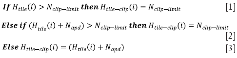
where Htile (i) is the histogram of the image tile (contextual region), Htile-clip (i) is the clipped histogram of the tile, Nclip-limit is the actual clip limit which is defined by

and Napd is the average number of pixels distributed into each gray level.
Step 3: The intensity values of the tile after histogram clipping is then transformed into the Rayleigh distribution. RCLAHE is based on a monotonic gray-level intensity transformation such that the cumulative output density should equal to the cumulative probability distribution of the input image. Mathematically, the output intensity level y is related to the input intensity level x by Rayleigh function given by
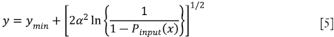
where ymin is the low bound, α is the Rayleigh parameter and Pinput (x) is the cumulative probability of the input image. Then, the output probability density can then be derived as
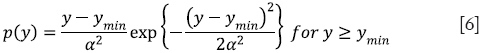
A higher Rayleigh parameter (α) value will result in more significant contrast enhancement in the image while at the same time increasing saturation and noise levels.
Step 4: The center point of tile is regarded as the sample point. The resulted mapping at each pixel is interpolated using bilinear interpolation of the neighboring sample points.
We have experimentally found that α ~0.45 was a good trade-off between contrast and noise in our OMAG images. Another parameter of RCLAHE is the saturation clip level which limits the CDF slope and the value of ~0.001 was experimentally chosen in our experiment.
In order to quantify the performance of our method besides visual validation, we utilized several quantities which can be divided into two categories: image quality measures and OMAG parameters which are explained below.
Image quality measures and quantities
Entropy
Entropy measures the content of an image, with higher values indicating more detailed images. The first-order entropy corresponds to the global entropy and is defined by
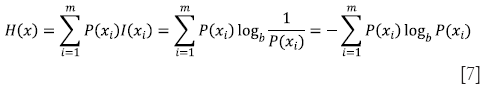
Where xi is an intensity value, m is the total number of intensity values in the dynamic range and P(xi) is the probability that a pixel in the image has an intensity value of xi.
Edge content-based contrast metrics (ECBCM)
Since human contrast sensitivity is highly dependent on spatial frequency, edge content-based contrast metrics (ECBCM) uses the concept of local band-limited contrast to simulate how human visual system processes information contained in an image. ECBCM of an area r is given by
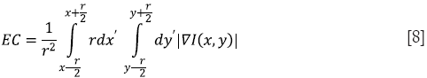
where ∇I(x,y) is the gradient (first-order derivative) of the image I(x,y). The formulation can be discretized in the form of

where m × n is the total number of pixels inside an area r (26).
Saturation evaluation
Saturation is defined as the percentage of saturated pixels (pure black or pure white) in an image.
Root-mean-square (RMS) contrast
Contrast is the difference in luminance that makes an object distinguishable from its background. It has many definitions but one of the most commonly used forms of contrast is root-mean square (RMS) contrast which is defined as
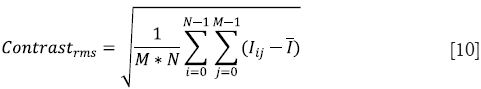
where Iij is the intensity of the image at pixel location (i,j),  is the average intensity of all intensity values in the image and M * N is the size of the image. Also, it is assumed that the intensity is normalized to the range [0,1].
OMAG parameters: vessel area density, vessel length fraction and fractal dimension
Most of the quantities defined above were common in any kind of image analysis and may not directly show any meaningful physiological parameter of vasculature map. Reif et al. (25) defined measurable parameters which could quantify OMAG images and were related to the physiological structure and location of the vessels. First, OMAG images are binarized using a threshold value. The vessel area density (VAD) is defined as the ratio of the number of white pixels (vessel) to the total number of pixels in the binary image. Then, the binary image is skeletonized (21) and the vessel length fraction (VLF) is defined as the ratio of white pixels to the total number of pixels in the skeleton image. Finally, the fractal dimension is calculated using a box counting technique (27) in the skeleton image. The box counting method divides the skeletonized image into equal-sized square tiles and counts the number of boxes containing a vessel segment. Through varying the box size, the process is repeated until the box size is equal to the image size. Then, the fractal dimension is defined using
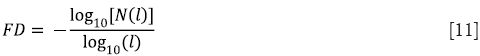
where l is the box length and N(l) is the number of boxes needed to cover the image. Both VAD and VLF have values in the range of [0,1] while FD has a value in the range of [0,2].
Experimental set up
To demonstrate the effectiveness of the proposed RCLAHE method in enhancing the imaging contrast while not affecting the metrics in terms of the microvasculature quantification, we used an OMAG imaging system to acquire the microvasculatural images within tissue beds in vivo, on which the algorithm is tested. In the OMAG/OCT system, we used a superluminiscent diode (SLD) with the center wavelength of 1,310 nm and bandwidth of 65 nm was used, delivering an axial resolution of ~12 µm in the air. An optical circulator was used to couple the light from the SLD into fiber-based Michelson interferometer. In the reference arm of the interferometer, a stationary mirror was utilized after polarization controller. In the sample arm of the interferometer, a microscopy objective lens with 18-mm focal length was used to achieve ~5.8 µm lateral resolution. Then, a 2×2 optical fiber coupler was utilized to recombine the backscattered light from the sample and the reflected light from the reference mirror. Since the wavelength of the light source is invisible to the human eye, a 633-nm laser diode was used as a guiding beam to locate the imaging position. This reference helps to adjust the sample under the OMAG/OCT system and image the desired location. The recombined light was then routed to a home-built high-speed spectrometer via the optical circulator. In the design of the spectrometer, a collimator with the focal length of 30 mm and a 14-b, 1,024-pixels InGaAs linescan camera (SUI, Goodrich Corp) were used. The camera speed was 47,000 lines per second and the measured SNR was ~105 dB with a light power on the sample at ~3 mW. The spectral resolution of the designed spectrometer was ~0.141 nm that provided a detectable depth range of ~3.0 mm on each side of the zero-delay line. The schematic of our imaging system is shown in Figure 2A and an image of a mouse ear pinna captured by a digital camera is shown in Figure 2B. The rectangle shown in Figure 2B is a typical field of view and scanning range for OMAG/OCT system, which is 2.2 mm × 2.2 mm in the current setup. In order to scan a larger field on the ear, we used a mechanical translating stage to move the tissue sample to the desired location and after acquisition and processing, the mosaics were stitched together to form a larger image.

Non-invasive in vivo images were acquired from the pinna of a healthy ~6 weeks old male hairless mouse (Crl:SKH1-Hrhr) weighting approximately 26 g. During the experiment, the mouse was anesthetized using 2% isoflurance (0.2 L/min O2, 0.8 L/min air). The ear was kept flat on a microscope glass using a removable double-sided tape. The experimental protocol was in compliance with the Federal guidelines for care and handling of small rodents and approved by the Institution Animal Care and Use Committee (IACUC) of the University of Washington, Seattle.
The scanning protocol was based on three-dimensional ultrahigh-sensitive optical micriangiography (UHS-OMAG) technique (9). The X-scanner (fast B-scan) was driven with a saw tooth waveform and the Y-scanner (slow C-scan) was driven with a step function waveform. The fast and slow scanners covered a rectangular area of ~2.2 mm × 2.2 mm on the sample. Each B-scan consisted of 400 A-lines covering a range of ~2.2 mm on the sample. The duty cycle of the saw tooth waveform rising edge was set at ~80% per cycle, which provided a B-scan frame rate of ~94 frames per second. The C-scan consisted of 400 scan locations with B-scan repetition of 8 frames per location for flow imaging and quantification. The total size of the data set was 1.28×10⁶ A-lines. In order to cover a large field of view, multiple 3-D scan were acquired and the sample was translated using a mechanical stage. This allowed imaging an area of ~1.5 cm × 1.5 cm on the mouse ear pinna.
The captured data was processed off-line using MATLAB© (MathWorks) which processed repeated B-scans at the same spatial location and generated cross-sectional vessel map using eigendecomposition-based (ED) filtering technique (14). Then, the adjacent cross-sections were visualized in a volumetric formation to show 3-D information and vessel map.
Results and discussions
Figure 3A shows a typical cross-section (B-scan) of the mouse ear pinna structure (near the edge). Figure 3B shows the processed ED-OMAG cross-section at the same location. Total 3-D data can be visualized in Figure 3C where vessels (labeled red) are overlaid on the structure (yellow), where the location of structure and vessel cross section of Figure 3A are marked as the dark line. After 3-D Gaussian filtering followed by median filtering, maximum intensity projection (MIP) map of the vessels are given in Figure 3D, showing the detailed microvascular network, including capillary vessels, that perfuses the scanned tissue volume. With the multiple mosaics of such MIP images acquired, the vasculature map of the entire mouse ear pinna is obtained by simply manually stitching them together. Two such stitched images are shown in Figure 1. All of the contrast enhancement, equalization methods and quantifications explained in this paper were performed on individual MIP images (mosaics).

Figure 4A shows OMAG microvasculature map of mouse ear pinna after stitching 22 projection map images (mosaics) without applying any post-processing to this image. It can be observed that the vessel signal background noise is not homogenous all over the ear due to imaging conditions, surface refraction and variations of light scattering properties. RCLAHE was applied to every single mosaic and then the mosaics were stitched together to form Figure 4B. It is obvious that the OMAG image is now homogenous everywhere, and signals from vessels has been improved while not saturated. Figure 4C shows one of the mosaics of Figure 4A where the vessel map and background is not homogenous, and Figure 4D shows RCLAHE enhanced mosaic. It can be observed that the contrast of the capillary loops on the ear edge has been improved. Also, the background has been suppressed while foreground has been amplified.

Similarly, Figure 5A shows OMAG microvasculature map of another mouse ear pinna after stitching 25 mosaics without any post-processing and after applying RCLAHE (Figure 5B). Also, Figure 5C shows one of the mosaics which had a high background due to high surface refraction which has been corrected in Figure 5D. It can be observed that the signal at the lower left corner of the ear pinna is poor, and the capillary loops have low contrast. These defects have been corrected using RCLAHE (Figure 5D).

In order to compare the performance of RCLAHE with other standard contrast enhancement and equalization methods, we applied contrast stretching algorithm (CSA), local histogram equalization (LHE), global histogram equalization (GHE) and uniform contrast limited adaptive histogram equalization (UCLAHE), respectively, to the mouse ear pinna mosaics and compared the results with RCLAHE both qualitatively and quantitatively. The parameters discussed earlier were used to quantify the performance of each method. Note that GHE is identical to LHE but the algorithm is applied to all of the mosaics at the same time. This procedure improves the general appearance of the image because it considers the histogram in all of the mosaics. Also, the ear edge mosaics that have a high background after LHE was corrected using GHE.
Figure 6A shows the original ear pinna image without any equalization, and Figure 6B-H show the performance of CSA, LHE, GHE, UCLAHE and RCLAHE methods on Figure 6A, respectively. The performance of each method on a selected mosaic can be observed where the mosaics are the result of no enhancement (Figure 6G), CSA (Figure 6H), LHE (Figure 6I), GHE (Figure 6J), UCLAHE (Figure 6K) and RCLAHE (Figure 6L) methods, respectively. Compared to the original image before enhancement (Figure 6A), CSA (Figure 6B) improves the contrast of the vessels but does not improve the signal strength at the vessel locations and some weak capillary loops are not improved. Also, the background at high surface refraction areas of ear was not improved. Although LHE (Figure 6C) improves and amplifies the vessels and capillary loops at the areas with weak signals, but has an artifact at the ear edge where the background noise has also been amplified. GHE (Figure 6D) does not have ear edge artifact but the vessels have been saturated and some weak vessels are still not obvious. Also, the heterogeneous background at high surface refraction areas is still obvious. Although UCLAHE (Figure 6E) overcame most of the limitations of its previous methods but the signal is still very weak at capillary loops and small vessels and the image contrast is very low. Also, the high surface refraction is not compensated either. RCLAHE (Figure 6F) creates a homogenous vasculature map all over the ear and improves the weak signal at capillary loops and small vessels as well as high surface refraction areas. Also, RCLAHE is less saturated than UCLAHE and better intensity distribution at larger vessels can be observed.

Table 1 shows the quantitative comparison of OMAG and image parameters in Figure 6A-F. It can be observed that LHE and GHE increased the mean intensity, RMS contrast and ECBCM of the original image while at the same time increased the saturation level especially at larger vessels. Although CSA method improved saturation level, other image parameters such as mean intensity, RMS contrast, ECBCM and entropy were reduced. UCLAHE improved mean intensity and RMS, RMS contrast and saturation level while the entropy and ECBCM were decreased. RCLAHE improved the image parameters. The entropy and RMS contrast of LHE and GHE were higher than RCLAHE, because the ear edge background was amplified and the vessel boundaries were saturated. More importantly, the OMAG parameters were very similar between different methods and most of methods slightly increase these parameters which was because of increasing the mean intensity of the images which allowed some weak vessel signal be also included in the quantification. UCLAHE had similar mean intensity value which made its OMAG parameters identical to the original image. Basically, the our analysis show that these contrast enhancement methods did not change physical appearance of the vessels and therefore OMAG parameters were similar in all cases.

Full Table
In order to show the performance of the implemented methods on only one mosaic image, the OMAG and image parameters of Figure 6G-L were compared in Table 2. In this mosaic (Figure 6G), the background of the image was and vessel intensities were not homogenous. Also, larger vessels were saturated and their distribution was flat. Except for LHE, other methods did not dramatically change the OMAG parameters. Although CSA method improved the saturation problem, its RMS contrast, entropy and ECBCM were lower than the original image. GHE obviously saturated the larger vessels image. Although UCLAHE solved saturation, it could not improve the heterogeneous background artifact and its entropy, ECBMC and RMS contrast were low. RCLAHE not only reduced the background artifact, it also increased RMS contrast, entropy and ECBCM without oversaturating the image.

Full Table
Similarly, Figure 7A-F show the qualitative comparison between different methods and their image and OMAG parameters are compared in Table 3. Also, the performance of different methods on a selected mosaic in Figure 7G are shown in Figure 7F-L and their quantities were compared in Table 4. The original image (Figure 7A) had some areas with weak signals and low contrast at capillary loops near the ear edge. Although CSA improved the local appearance and contrast of the image at some areas, the overall picture was heterogeneous and some week signal vessels were not amplified because they were in the same mosaic of some stronger signals. LHE and GHE improved the contrast and mean intensity while both methods saturated the image and LHE had similar artifacts at ear edges and GHE could not compensate the high surface refraction. UCLAHE could not improve the background artifact at low intensity capillary loops near the ear edge and its overall appearance was not homogeneous. RCLAHE solved the low artifact at low intensity capillary loops and edges while preserving the saturation level. It also improved other parameters such as RMS contrast, ECBCM and entropy. OMAG parameters were larger than the original image because weak signal capillary loops fell below segmentation threshold and after RCLAHE processing; these loops were also included in OMAG parameter analysis.

Full Table

Full Table

Conclusions
In this paper, we proposed using RCLAHE to improve the contrast and overall appearance of OMAG without saturating the vessels. The qualitative and quantitative performance of the proposed method was compared with those of CSA, LHE, GHE and UCLAHE. It has been demonstrated that RCLAHE outperformed LHE and GHE while at some local areas it was similar to CSA and UCLAHE. However, the overall performance was relatively better, and RCLAHE was the only method to overcome the heterogeneous background artifact. This post-processing can be applied in applications which require imaging a larger than the system field of view area or when inhomogeneous background surface refraction variations exist. OMAG parameters such as vessel density and fractal dimension were similar in most of the methods which confirmed that contrast enhancement methods did not change physical meaning of the image and only the overall appearance was different which an observer can decide which methods works best for a particular application. This method is not limited to optical microangiography and can be used in other image modalities such as photo-acoustic tomography and scanning laser confocal microscopy.
Acknowledgements
This work was supported in part by research grants from the National Institutes of Health (R01HL093140, R01HL093140S, R01EB009682 and R01DC01201) and the W.H. Coulter Foundation Translational Research Partnership Program. Dr Wang is a recipient of Research to Prevent Blindness Innovative Research Award. The content is solely the responsibility of the authors and does not necessarily represent the official views of grant-giving bodies.
Disclosure: This manuscript has not been submitted or published anywhere else. The authors have no financial interest in the information contained in the manuscript.
References
- Wang RK, Jacques SL, Ma Z, et al. Three dimensional optical angiography. Opt Express 2007;15:4083-97.
- Misgeld T, Kerschensteiner M. In vivo imaging of the diseased nervous system. Nat Rev Neurosci 2006;7:449-63.
- McDonald DM, Choyke PL. Imaging of angiogenesis: from microscope to clinic. Nat Med 2003;9:713-25.
- Molina CA, Saver JL. Extending reperfusion therapy for acute ischemic stroke: emerging pharmacological, mechanical, and imaging strategies. Stroke 2005;36:2311-20.
- Imai M, Iijima H, Hanada N. Optical coherence tomography of tractional macular elevations in eyes with proliferative diabetic retinopathy. Am J Ophthalmol 2001;132:81-4.
- Martin P. Wound healing--aiming for perfect skin regeneration. Science 1997;276:75-81.
- Wollstein G, Paunescu LA, Ko TH, et al. Ultrahigh-resolution optical coherence tomography in glaucoma. Ophthalmology 2005;112:229-37.
- Hee MR, Baumal CR, Puliafito CA, et al. Optical coherence tomography of age-related macular degeneration and choroidal neovascularization. Ophthalmology 1996;103:1260-70.
- An L, Qin J, Wang RK. Ultrahigh sensitive optical microangiography for in vivo imaging of microcirculations within human skin tissue beds. Opt Express 2010;18:8220-8.
- Wang RK. Three-dimensional optical micro-angiography maps directional blood perfusion deep within microcirculation tissue beds in vivo. Phys Med Biol 2007;52:N531-7.
- Wang RK. Directional blood flow imaging in volumetric optical microangiography achieved by digital frequency modulation. Opt Lett 2008;33:1878-80.
- Wang RK, An L, Francis P, et al. Depth-resolved imaging of capillary networks in retina and choroid using ultrahigh sensitive optical microangiography. Opt Lett 2010;35:1467-9.
- Qin J, Jiang J, An L, et al. In vivo volumetric imaging of microcirculation within human skin under psoriatic conditions using optical microangiography. Lasers Surg Med 2011;43:122-9.
- Yousefi S, Zhi Z, Wang R. Eigendecomposition-Based Clutter Filtering Technique for Optical Micro-Angiography. IEEE Trans Biomed Eng 2011;58:2316-23.
- An L, Shen TT, Wang RK. Using ultrahigh sensitive optical microangiography to achieve comprehensive depth resolved microvasculature mapping for human retina. J Biomed Opt 2011;16:106013.
- Jia Y, Li P, Wang RK. Optical microangiography provides an ability to monitor responses of cerebral microcirculation to hypoxia and hyperoxia in mice. J Biomed Opt 2011;16:096019.
- Zhi Z, Jung Y, Jia Y, et al. Highly sensitive imaging of renal microcirculation in vivo using ultrahigh sensitive optical microangiography. Biomed Opt Express 2011;2:1059-68.
- Miles KA, Lee TY, Goh V, et al. Current status and guidelines for the assessment of tumour vascular support with dynamic contrast-enhanced computed tomography. Eur Radiol 2012;22:1430-41.
- Tan TL, Sim KS, Tso CP, et al. Contrast enhancement of computed tomography images by adaptive histogram equalization - application for improved ischemic stroke detection. Int J Imag Syst Tech 2012;22:153-60.
- Pisano ED, Cole EB, Hemminger BM, et al. Image processing algorithms for digital mammography: a pictorial essay. Radiographics 2000;20:1479-91.
- Gonzalez RC, Woods RE. eds. Digital image processing. Houston: Prentice Hall, 2002:519-32.
- Pizer SM, Amburn EP, Austin JD, et al. Adaptive histogram equalization and its variations. Computer vision, graphics, and image processing 1987;39:355-68.
- Pizer SM, Johnston RE, Ericksen JP, et al. Contrast-limited adaptive histogram equalization: speed and effectiveness. Proceedings of the First Conference on Visualization in Biomedical Computing 1990:337-45.
- Zuiderveld K. Contrast limited adaptive histogram equalization. In: Paul S. eds. Graphics gems IV. Boston: Academic Press Professional, Inc., 1997:474-85.
- Reif R, Qin J, An L, et al. Quantifying optical microangiography images obtained from a spectral domain optical coherence tomography system. Int J Biomed Imaging 2012;2012:509783.
- Saleem A, Beghdadi A, Boualem B. Image fusion-based contrast enhancement. EURASIP Journal on Image and Video Processing 2012;1:10.
- Masters BR. Fractal analysis of the vascular tree in the human retina. Annu Rev Biomed Eng 2004;6:427-52.

