
Experimental method and statistical analysis to fit tumor growth model using SPECT/CT imaging: a preclinical study
Introduction
Oncology imaging is performed using various modalities including computed tomography (CT), magnetic resonance imaging (MRI), single-photon emission computed tomography (SPECT) and fluorodeoxyglucose-positron emission tomography (FDG-PET).Quantification of cancer from images is important for assessment of disease progress and treatment. Tumors grow in a specific way and theoretical tumor-models of increasing complexity have been developed that may be potentially used to find (otherwise concealed) biophysical information from serial images of tumors. If accurate, tumor growth-rate, cell-motility (diffusion), tumor-necrotic-factor, can be consistently and reliably extracted from oncological images, they may add valuable information on the tumor containment/spread and help treatment plan. For example, assessing the growth-rate accurately will help in treatment planning whether in surgery or in determining the number of fractions and dose of radiotherapy. Biological research shows tumor-necrotic-factor may have a stabilizing effect on proliferating cells (1). Applying equations to images of tumor density, accounting for cell-motility and proliferation of glioma tumors have shown promise in therapy evaluation, as well as in vitro analysis (2-4), and has been used to register patient scans to brain atlas (5,6).
However, research on in vivo image analysis using mathematical models-fitting image datasets (clinical or even pre-clinical) to extract quantification parameters for subject-specific tumor-characterization is sparse. Recently pre-clinical experiments to predict volume (7) and metastasis (8) have been performed. In (7) several classical existing tumor-volume growth models (such as logistic, Gompertzian etc.) were considered and compared with extracted breast-and lung tumor volumes of mice measured with calipers. For the breast data, the dynamics were best captured by the Gompertzian and exponential-linear models (with predictive scores of ≥80%). For lung-tumor Gompertz and power-law prediction was best, however with prediction rate ≤70% and required prior information on parameter distribution to improve. In (8) primary and metastatic tumor growth models were compared with measurements from preclinical images of breast-tumor bearing mice, with mixed results: coefficients of determination were R2=0.94 for primary tumors but only R2=0.57 for metastatic growth. Key parameter extraction such as diffusion coefficient, growth rate of gliomas was performed on simulated and in vivo preclinical images in (9). While the simulation results showed low errors, in vivo experimental studies showed lower predictive accuracy. With the authors suggesting that including intra-tumor effects such as necrosis might improve experimental results. Indeed, none of these models in (3-9) explicitly incorporate tumor necrosis. However, most tumors beyond a certain diameter (~2–5 mm) develop necrotic cores, due to lack of nutrient (10-12). Thus necrosis formation is an important factor to be accounted for in serial images to obtain accurate parameters such as growth-rate. Necrosis effects have been modeled theoretically by moving boundary methods modeling nutrient concentration (mainly by oxygen diffusion) (13-17), but on the other hand, in these models, typically, tumor cell density or volume effects (6-7,18) are not explicitly considered.
Another model that incorporates necrosis is the theoretical ode-compartment volume model proposed by Wallace and Guo (18). In this model, the tumor is assumed to be composed of concentric shells of proliferating (P) and quiescent layers (Q) with a necrotic core (N). The Wallace-Guo model considers an overall effect of necrosis on the proliferating layer and may provide a more accurate picture of tumor proliferation than models which do not consider necrosis. Several different combinations of growth and necrosis models are proposed in theory in (18) and while some are forward simulated, none are fitted to any experimental data.
In the current work, the theoretical Wallace-Guo model (18) for tumor-growth is investigated using in vivo images of tumor-bearing mice. The reasons we chose this model is that it is comprehensive (with inclusion of classical growth-models, necrosis and cross-dependence thereof), yet simple and robust, making it particularly amenable for use in a clinical setting. In addition, being a volume model, it does not require explicit voxel-wise correspondence or accurate co-registration of data across different time-points that will be required for density models. This might be particularly important in a clinical setting with several months intervening between scanning of patients during which time there could be significant weight loss and other changes in body.
From experimentally acquired mice-tumor images, typically a quiescent layer cannot be reliably distinguished from the necrosis layer. Therefore, to enable our in vivo analysis, we made some small modifications to the main structure of the theoretical model in (18) to obtain a two-compartment version, to better fit the experimental data. Also, in addition to the surface-area based and logistic growth considered in (18), we added for consideration a Gompertzian growth because of its strong results for in vivo use (7).
In the following sections, we develop an inversion algorithm for fitting the models, which we test in simulated datasets as well as in vivo experimental images. For the simulated datasets, we first generated volume data according to model equations. After corrupting our generated volumes with noise, we perform an assessment in the error of our parameter recovery. Then, we fit the experimental in vivo mice-tumor data by the two-compartment models. We conclude by presenting the results of the Akaike information criterion (AIC) evaluations on the models.
Methods
Mathematical model and its variants
Mathematical model and variations used
Eqs. [1-3] shows one of the systems of non-linear differential equations proposed by Wallace and Guo (18) that attempts to capture the dynamics of tumor growth. This three-compartment model includes a Proliferating (P) region, a Quiescent (Q) region, and a Necrotic (N) region. The model captures the interdependence of the different cell pools that make up a tumor with different combinations of functions for growth with other terms considered. In (18), of the 25 different models explored, the one designated 3E was concluded to perform the best, given in the following equations.
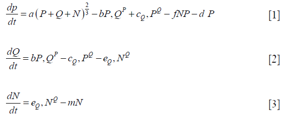
Note that the growth term in Eq. [1(a)] is proportional to surface area of the tumor volume. The α is the growth-rate parameter, bP,Q defines the rate-factor at which the P-cells becomes Q-cell (reducing  and
and  increasing) and cQ,P defines the rate at which Q-cells become P-cell. The eQ,N defines the necrosis rate of the Q-cells. The f takes into account the effect of the N on P, where the necrotic region releases substances that reduces the proliferation rate. This is expected to be related to the Tumor-Necrosis-Factor (TNF). This effect depends on the volume of N as well as P. Understandably this affects only the proliferating cells. The d and m are the self-slow-down rate of proliferation and necrosis respectively. Treatment terms maybe incorporated into parameter d.
As mentioned, it will be challenging to distinguish between the Q and the N layer from our acquired SPECT/CT images, (or clinical images over the long-term). Thus for the experimental case, we modified the model to a two-compartment (P-N) approximation of Eqs. [1-3], shown in Eqs. [4,5]. Note that the eP,N describes the (one-way) process of proliferating cells becoming necrotic and the corresponding growth of necrotic shell. The G(P) is a general growth function.
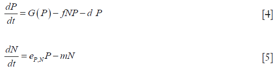
While remaining within this Wallace-Guo compartmental framework, we also used other forms of the function G(P), which is in control of the growth of the proliferating cells. This is motivated by the fact that in vivo tumors will show different characteristics than spheroids, with growth less dependent on outer surface-area and will have other population-death characteristics. This gives us three new models, as described below.
Model A: assumes that growth is proportional to the surface area of a spheroid (as in Eqs. [1-3] 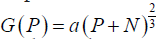 :
:
Model B: utilizes the logistic function to limit the growth of P: G(P)= aP – bP2
Model C: utilizes the Gompertzian function to limit the growth of P: G(P)=ae(–bt)P
Iterative model inversion
Volume data P, Q, N or where appropriate just P and N, were fitted to our candidate models by iteratively minimizing their weighted residual sum of squares. The weighted sum square allows us to weight compartments differently when one becomes disproportionately large and dominates the minimization. For example, if the necrotic layer is too large, unless weighted, it will dominate the sum-squared-error and might yield results with higher model-fitting errors in other compartments. At the n-th iteration, with parameter set ϕn, let Mc (t, ϕn) be the output of the c-th compartment of the model M (t, ϕn), where c denotes P,Q,N (Eq. [1]) or P,N (Eq. [2]). The weighted sum squared error, as denoted by the quantity WRSS below is then iteratively minimized:
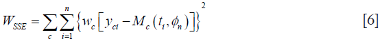
where wc is an optional weighting factor for each of the thee (or two) compartments P,Q,N (or P, N), yci represents the measured volume data obtained at time ti, via experiments or simulations, and M (ti, {ϕn}) is the value predicted by the model. ϕ is a best fit parameter if it minimizes WSSE, and the resulting best-fit parameter vector is denoted by . Minimization of the WSSE was performed by MATLAB (MathWorks, MA, USA) function fmincon, which minimizes non-linear multivariable functions.
Assessment of inversion algorithm using simulated data
In order to assess our inversion algorithm, we corrupted the forward-model simulation of Model A with 30 cases of realistic additive Gaussian noise and inverted the model at three selective time points. This allowed us to examine how well the inversion algorithm recovered the parameters compared to the true parameters. We began by solving the three-compartment model given by Eqs. [1-3]. The system of ordinary differential equations was solved using the ode 45 function, in Matlab. The solution was then corrupted with additive Gaussian noise. To make this Gaussian noise realistic, it was made proportional to the segmentation error, in particular, the mean of the partial volumes ΔV+ and ΔV– which are the overestimated and underestimated compartment volumes by 1 pixel error on either side of the boundary. This reflects realistic errors we encountered when segmenting experimental data. Thirty noise realizations were simulated.
Experimental image acquisition and image processing
Mice experiments and ethics
Three immunodeficient female NSG mice were injected with 4T1-hNIS breast cancer cell line from Imanis Life Sciences, engineered to overexpress the sodium iodide symporter (NIS) gene. They were then injected with Tc99m and imaged three times (with at least a 3-day interval for a near-complete decay of Tc-99m) with Flex Triumph Micro-SPECT/CT located in Mathis’s lab, SVM, Louisiana State University (LSU). The experiment was repeated with seven additional mice of which only three had usable datasets with 3 time-points each. All the experiments were conducted with strict adherence to protocols approved by the Institutional Animal Care and Use Committee (IACUC) within LSU. The animals were monitored every other day for pain/distress and a scoring system was utilized to prevent unnecessary pain/distress. Animals that showed pain and/or distress and/or exhibited significant tumor burden, significant weight loss (i.e., cachexia greater than 20% of initial body weight), tumor ulceration, or impairment were euthanized by asphyxiation with CO2. Only one animal had to be euthanized after the two time points due to significant tumor-burden before she showed any signs of distress. At the end of the 3 time-points, all the animals were euthanized. From the two sets of experiments, we had total of six mice datasets with 3 time-points each to fit our models.
No. of time points: due to the 3-day imaging delay required for Tc99m decay before re-injection and strict IACUC protocols to euthanize the animals before significant tumor-burden, more than three-time points were infeasible for this particular type of tumor.
Segmentation of volumes
The segmentation steps are shown in Figure 1. The proliferating (P) layer volumes were semi-automatically segmented from SPECT images in 3D using ITK-SNAP (19,20), see Figure 1A. The segmentation chosen was the semi-automatic 3D segmentation method. The choice of automated 3D segmentation was motivated by initial slice-by-slice hand-segmentation of boundaries, causing un-evenness in direction orthogonal to slices. The segmentation method in ITK-SNAP was smooth with similar levels of accuracy in all directions and thus preferred over hand-segmentation. The threshold to distinguish necrosis versus viable tumor cells (the input parameter to ITK-SNAP) was chosen via SPECT image histogram analysis over the tumor region in ImageJ. As shown in Figure 1B a contour was drawn including the boundary between the two regions. The threshold value was then chosen at the minima in the histogram that separated the intensities in the two zones. In all 18 cases (6 mice, 3 time-points) there was a clear minimum in the histogram that correlated well with the boundary gradient. Figure 1A shows an example-segmented tumor (in red). The volume-segmentation was done by the same person (Megan E. Chesal), for consistency.

The engulfed necrotic regions inside the tumors were segmented using our own software. Figure 1C uses a combination of morphological “closing” and connected-component analysis on difference image. Our simple, but robust, method works for these complex cases where proliferation and necrotic layers are topologically complex with necrotic volumes interconnected in tunnels and/or has multiple disjointed regions. The segmented P- and N-layer volumes are then used in model-fitting.
Goodness-of-fit criterion across different models
To judge the good-ness of fit of the models, one of the metrics we considered was the coefficient of determination or the R2 statistic. The R2 statistic measures how close the fitted regression line approximates the data. The R2 statistic was acquired with MATLAB’s built-in function fitlm. An R2 value close to 1 indicates that most of the variability in the data can be explained by the model M. To calculate this measure, we considered all the measured time-points for all the experimental datasets. For example, for the experiments with mice (described in later section in details), with 6 mice at 3 time points, the regression fit between the model and the experiments was done using all 6×3=18 time points.
Since increasing the number of independent variables in a model can only increase the R2 value (which can lead to R2 inflation), we included another fitting metric, capable of acting as a safeguard to overfitting. This metric is the AIC (21,22):
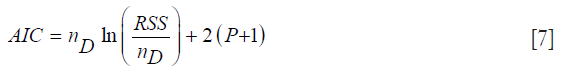
where nD is the number of data points, and P is the size of the parameter vector. The quantity P+1 will be denoted as k. The RSS is the residual sum-squared data between the model and measurement over all the measurement time-points over both layers P and N. The AIC rewards goodness-of-fit; but it also penalizes models for adding extra parameters, thereby discouraging overfitting. The model with the minimum AIC value is the preferred model from a set of candidate models.
Since the AIC is at times prone to choosing more complex models when nD is not that much larger than k2, (which is true for our case) we also consider the corrected version of the AIC which is denoted as AICc (21,22):
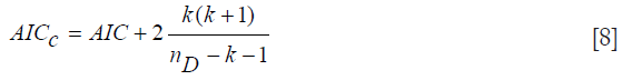
The AICC is more stringent in the sense that it exhibits harsher penalization for adding extra parameters, and it converges to the value of the AIC when nD gets larger. Both the AIC and AICc are used to select the “best” Kullback-Leibler model from a set of different candidate models suited for the given data. Once the “best” model is selected, further comparisons can be made between it and the other models by considering the Akaike differences and the Akaike weights. The Akaike difference is denoted as ΔAICC (21,22):

where AICCi denotes the AIC value for model i and AICCmin the minimum of the AICC values for the M different models. The “best” model, of course, has Δi=0. If a model has Δi less than 7, it has plausible support. If it has Δi between 7 and 11, it has little support, and any model with Δi greater than 14, has essentially no support and is considered implausible. The Akaike weights are denoted as wi (21,22):
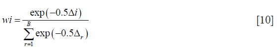
The Akaike weight of a model is that model’s probability of being the K-L “best” model among the set of candidate models. Notice how the sum of all the weights will always equal 1. These weights can help quantify the uncertainty of the model selection process.
Results
Simulations: parameter (or feature) recovery in presence of noise
In order to assess our inversion algorithm we simulated 30 realization of Forward model of Eqs. [1-3], as described previously in the section for assessment of inversion algorithm. We used parameters recommended by Wallace-Guo (18). However, we changed the m parameter in Eqs. [1-3] to have a small non-zero positive value (to be realistic). All this does is make the N-layer settle down at a specific equilibrium value, as expected in vivo. We then fitted the model by minimizing the weighted sum squared error of P, Q, N using MATLAB’s fmincon function as described in Methods section.
Figure 2A shows the forward simulations without added noise. Figure 2B shows the random realization of P (added noise) and its corresponding fitted value. We chose to fit 3 time-points to be consistent with mice data acquired (as explained in Experimental Section in Methods).

The simulations are unit-less to adapt to different experimental conditions/cases as in (18). However, time-units in hours and volume-units in 50 mm3 would approximately scale the axes to adapt to our mice experiments.
Figure 3 shows a bar chart of the true parameters and the average mean-parameters with standard-error bar. Note that the parameters are denoted in shorthand, such as eqn instead eQ, N of for simplicity and clarity of display. Also, not all the parameters are annotated for clarity, but from left to right the bars correspond to parameters a, bpq, cpq, d, eqn, f, m.

In Table 1 we show the true parameters and followed by the statistics of the recovered parameters for 30 noise-realizations: the mean, %-error, standard deviation (STDV), Standard error (SE). The results show that 5 of the 7 parameters can be recovered to have errors less than 4.3%. In particular, the useful feature of growth-rate (parameter a) is recovered with less than 0.07% error. The remaining two parameters (f and m) were related to the necrosis and had higher percentage errors. The parameter m, which affects the necrotic volume, was very small in magnitude and difficult to estimate from noisy-data. This had a ripple effect on f, a potentially useful feature related tumor-necrotic-effect, increasing its error to 7.8%. On the whole, the results indicate that 6 out of 7 features could be extracted to within ~7.8% error.

Full table
Mice data fitting for different models
The mouse-data fits for all six mice yielded visually reasonable results. Even though each model had different fitting errors, interestingly the best and the worst cases were always the same two mice respectively for all the models, qualitatively and quantitatively. The reason for this is likely due to low or high segmentation error. Figure 4 shows an example fitting for the mouse, Model A, B and C. The fitting of Models B and C were quantitatively different but visually nearly indistinguishable for many cases.

Goodness of fit of mice data for different models
Figure 5A,B,C show the regression fits with 95% confidence intervals (dashed-lines) for P and N layer with 6×3=18 data points (6 mice at 3 time-points) for the three models. Qualitatively the linear-regression describes the predicted and observed P- and N-layers well. For the N-layer, the errors were relatively higher than P-layer. Models B and C have R2 of 0.99 for P layer and Model A has 0.96. For the N-layer the R2 values were 0.95, 0.93 and 0.94 respectively for surface-area, logistic and Gompertzian. As far as the P-layer volume prediction is concerned, which is of most interest to us, the Model B and C performances were superior to Model A. Finally, in Table 2 we report the AIC analysis for model-comparison. All metrics pointed to surface-area (Model A) performing worse over Model B and C. The RSS (root-mean-squared error over all 18 data-points and all layers), AICc, AIC, and ∆AIC were highest for Model A. The AIC-weight in particular seemed to eliminate the surface-area as a good predictor of in in vivo data, with the weight near-zero. The performance of Model B (Logistic) and C (Gompertzian) was similar with the Gompertzian slightly better than Logistic. Since the AIC-weights were close, 0.43 and 0.57 for Logistic and Gompertzian, indicating both are plausible, both will be investigated in the future on clinical datasets.


Full table
Discussion
We have shown a method to extract potentially useful biophysical parameters from images of mice-tumors (without therapy). There is a wealth of information in the clinical patient datasets such as PET/CT, SPECT/CT or MRI, which can potentially be tapped. The model fitting will help characterize the tumors (such as accurate growth rate, TNF factor), which in turn may help decide the fractionation dose in radiation therapy and dose/cycle in chemotherapy. It is possible to generalize the approach to be applicable to datasets before and after therapy by including a time-dependent therapy effect terms {similar to the “d” in Eqs. [1,2], except time-dependent}.
We have performed our investigation on SPECT/CT datasets. However, other modalities such as MRI maybe considered for fitting these models, as in (5-7).
One of the limitations of this work is being able to acquire only 3 time-points due to the high-growth rate for the chosen tumor type, dose, imaging time constraints and IACUC requirements. In general, more time points will sample and capture the variations in the volume (or density) better. However, one mitigating factor is the strong constraints due to the ode-model with its cross-dependence on P and N. The P and N measurements provide two measured points to fit the model-constraint for each time-point. Indeed, our simulation results indicate that 3 time-points (provided spaced apart adequately) yields good accuracy. Note, in large-hospital clinical settings, 3–10 time-points, (with average of 5 time-points) is common for serial PET/CT datasets.
Since the model considered is a volume model, heterogeneity information of the tumor will be averaged out. We are currently building a FEM density model to account for tumor heterogeneity effects (23). FEM models can describe the high deformation of the domain necessary for tumor-growth. However, application of FEM models require accurate correspondence of voxels across different time points and hence co-registered data across different time points (via structural information in CT or MRI datasets). In contrast, the models considered have the simplicity of requiring us to consider only the functional modality (SPECT).
Conclusions and future work
We inspected three variants of the Wallace and Guo model for their goodness-of-fit on mice SPECT/CT datasets with 3 time-points. This is the first time the Wallace-Guo compartment model is used in vivo. Our results demonstrate that the Gompertzian growth model predicted the overall data most accurately for the six-mice datasets with 3 time-points each, with Logistic model closely following. The surface-area model predicted the in vivo data least well of the three. All three models included tumor necrosis factor and growth; our findings thus give us a perspective on how tumor growth ode models can be applied to in vivo experiments can provide useful parameters.
In the long-term we will investigate efficacy of the parameters of the volume model considered here and our density FEM model (23) for disease and treatment quantification in pre-clinical and clinical studies.
Acknowledgements
The authors wish to thank the Department of Physics & Astronomy and the College of Science, LSU for funding this work.
Footnote
Conflicts of Interest: The authors have no conflicts of interest to declare.
Ethical Statement: The experiment was repeated with seven additional mice of which only three had usable datasets with 3 time-points each. All the experiments were conducted with strict adherence to protocols approved by the Institutional Animal Care and Use Committee (IACUC) within LSU.
References
- Sedger LM, McDermott MF. TNF and TNF-receptors: From mediators of cell death and inflammation to therapeutic giants - past, present and future. Cytokine Growth Factor Rev 2014;25:453-72. [Crossref] [PubMed]
- Swanson KR, Bridge C, Murray JD, Alvord EC Jr. Virtual and real brain tumors: using mathematical modeling to quantify glioma growth and invasion. J Neurol Sci 2003;216:1-10. [Crossref] [PubMed]
- Swanson KR, Alvord EC Jr, Murray JD. A quantitative model for differential motility of gliomas in grey and white matter. Cell Prolif 2000;33:317-29. [Crossref] [PubMed]
- Swanson KR, Alvord EC Jr, Murray JD. Virtual brain tumours (gliomas) enhance the reality of medical imaging and highlight inadequacies of current therapy. Br J Cancer 2002;86:14-8. [Crossref] [PubMed]
- Hogea C, Davatzikos C, Biros G. An image-driven parameter estimation problem for a reaction–diffusion glioma growth model with mass effects. J Math Biol 2008;56:793-825. [Crossref] [PubMed]
- Gooya A, Biros G, Davatzikos C. Deformable registration of glioma images using EM algorithm and diffusion reaction modeling. IEEE Trans Med Imaging 2011;30:375-90. [Crossref] [PubMed]
- Benzekry S, Lamont C, Beheshti A, Tracz A, Ebos JM, Hlatky L, Hahnfeldt P. Classical mathematical models for description and prediction of experimental tumor growth. PLoS Comput Biol 2014;10:e1003800. [Crossref] [PubMed]
- Hartung N, Mollard S, Barbolosi D, Benabdallah A, Chapuisat G, Henry G, Giacometti S, Iliadis A, Ciccolini J, Faivre C, Hubert F. Mathematical modeling of tumor growth and metastatic spreading: validation in tumor-bearing mice. Cancer Res 2014;74:6397-407. [Crossref] [PubMed]
- Hormuth DA 2nd, Weis JA, Barnes SL, Miga MI, Rericha EC, Quaranta V, Yankeelov TE. Predicting in vivo glioma growth with the reaction diffusion equation constrained by quantitative magnetic resonance imaging data. Phys Biol 2015;12:046006. [Crossref] [PubMed]
- Hall EJ, Giaccia AJ. Radiobiology for the Radiologist. Lippincott Williams & Wilkins, 2006.
- Britton NF. Essential Mathematical Biology. London: Springer-Verlag London, 2003.
- Murray JD. Mathematical Biology. Springer, 2007.
- Cristini V, Lowengrub J, Nie Q. Nonlinear simulation of tumor growth. J Math Biol 2003;46:191-224. [Crossref] [PubMed]
- Cui S, Friedman A. Analysis of a Mathematical Model of the Growth of Necrotic Tumors. J Math Anal Appl 2001;255:636-77. [Crossref]
- Cui S, Friedman A. Analysis of a mathematical model of the effect of inhibitors on the growth of tumors. Math Biosci 2000;164:103-37. [Crossref] [PubMed]
- Escher J, Matioc AV, Matioc BV. Analysis of a mathematical model describing necrotic tumor growth. Springer Berlin Heidelberg 2011;57:237-50.
- Bearer EL, Lowengrub JS, Frieboes HB, Chuang YL, Jin F, Wise SM, Ferrari M, Agus DB, Cristini V. Multiparameter computational modeling of tumor invasion. Cancer Res 2009;69:4493-501. [Crossref] [PubMed]
- Wallace DI, Guo X. Properties of tumor spheroid growth exhibited by simple mathematical models. Front Oncol 2013;3:51. [Crossref] [PubMed]
- Yushkevich PA, Piven J, Hazlett HC, Smith RG, Ho S, Gee JC, Gerig G. User-guided 3D active contour segmentation of anatomical structures: significantly improved efficiency and reliability. Neuroimage 2006;31:1116-28. [Crossref] [PubMed]
- Available online: http://www.itksnap.org/pmwiki/pmwiki.php
- Burnham KP, Anderson DR, Huyvaert KP. AIC model selection and multimodel inference in behavioral ecology: some background, observations, and comparisons. Behav Ecol Sociobiol 2011;65:23-35. [Crossref]
- Mazerolle MJ. Making sense out of Akaike’s Information Criterion (AIC): its use and interpretation in model selection and inference from ecological data. Université Laval, Québec, Québec 2004.
- Dey J, Walker SW, Mathis JM, Shumilov D, Kirby KM, Luo Y. Modeling and analysis of a physical tumor model including the effects of necrotic core. Nuclear Science Symposium and Medical Imaging Conference (NSS/MIC), 2015 IEEE.

