
Analyzing bone remodeling patterns after total hip arthroplasty using quantitative computed tomography and patient-specific 3D computational models
Introduction
Total hip arthroplasty (THA) is one of the most widely performed surgeries in orthopaedics. First performed in 1960, THA has been remarkably successful in eliminating pain and allowing patients to regain the level of activity similar to the normal hip. Despite its success, adverse bone remodelling around the implant remains as one of the main causes for implant failure. As such, there have been a large number of clinical studies aiming to investigate bone remodelling patterns around the implant. These studies have used various imaging modalities such as DEXA or quantitative computed tomography (QCT) (1,2). However, bone density alone cannot be used as a major indicator for bone quality (3). Structural aspects such as micro architecture need to be considered too.
As a result, research is actively being undertaken to develop theoretical models, which are capable of predicting bone quality around implants after THA in the form of a bone remodelling algorithm. In particular, finite element analysis run in conjunction with bone remodelling algorithm is extensively used in these predictions. The practical importance of these mathematical models in pre-clinical testing was demonstrated in previous studies (4-7).
Bone quality can be obtained by bone density together with micro-architecture and a structural aspect from CT scans. Finite Element models can integrate these factors by incorporating bone material properties obtained from CT scans along with the external loads to examine the bone quality and its remodelling capabilities (8). In particular, patient specific finite element models can be created using geometrical and density information from QCT data sets obtained from osteodensitometry studies (9-12). Our previous work showed the combination of QCT and finite element modalities, hence improving the ability of FE models to monitor changes in bone architecture (with respect to stress patterns over time) and assess bone quality after total hip replacement (13).
Our aim in this study is to develop patient-specific finite element models from the patients’ own QCT scans and analyse their bone density change patterns over the 5-year post-op period. Total five regions of interest were chosen from the femur and then subdivided into four quadrants for quantitative analysis. Bone density change patterns in those regions were analysed in detail for cortical and cancellous bone separately over the 5-year period.
Materials and methods
All patient data (for post-operative, after 1, 2 and 5 years follow-ups) used in this study are taken from a QCT assessment study by Pitto and colleagues (9-11). It includes 29 patients (31 hips) with degenerative joint disease. All patients have received uncemented THA with a taper design femoral component (Summit, DePuy International, Leeds, UK) and press-fit titanium cup (Duraloc; DePuy) with ceramic-ceramic pairing (Biolox Delta, ceramTec, Plochingen, Germany). The average age of a patient at the index operation was 58 years (range, 31-81 years). There were 16 males and 13 females. All patients were operated by the same surgeon. Four patients are analysed and the bone remodelling patterns are compared in this study. Those patient’s gender and age are as follows, Patient 1—Female 81 years old, Patient 2—Male 58 years old, Patient 3—Male 64 years old and Patient 4—Male 49 years old.
Two types of CT machines are used to obtain CT images, Philips Brilliance 64 and Siemens Somatom Plus 4. Acquisition parameters were remained the same for both machines. Tube voltage was 140 kVp, tube current was 206 mAs and slice thickness was less than 2 mm, which produced images with the resolution of 0.29 mm. These QCT images are examined to obtain the geometry and the bone density information of the femoral components. They are segmented using an image processing software, Image J 1.46r (by National Institute of Health, USA) as shown in Figure 1. A synthetic phantom containing a circular sample with defined HA concentration was scanned during every examination for conversion of Hounsfield units (HU) into hydroxyapatite (mgCaHA/mL) equivalents. This operation was required to convert radio-logical bone density to true bone mineral density.

Image segmentation is performed manually at this stage. Although we have developed an automatic algorithm for image segmentation in the past (12), the presence of metal artefacts made it difficult to use the automatic algorithm without further manual correction, which did not improve the overall efficiency. Therefore we have used a manual procedure for image segmentation. Once segmentation was completed, QCT image stack of each follow-up is aligned in 3D according to the image position information recorded in the respective header file. Bone density value at each point of the QCT image is extracted according to the Hounsfield equation as shown in Eq. [1].

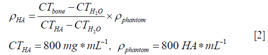
Rescale slope and rescale intercepts are designed parameters, obtained from CT machine. Then, Hounsfield values are converted to bone density values in mg*mL−1 by using the calibration Eq. [2] given below (12). A hydroxyapatite phantom with a known density of 800 HA*mL−1 is scanned after scanning each patient and stored as and CT phantom.
Next, resulted 3D data set of each follow-up is realigned to the post-operative 3D data set in graphical user interface of our software called CMGUI (version 2.9.1, freely available for academic use at www.cmiss.org). Bone density input file of the respective follow-up is generated by using those new transformation values and the Hounsfield values. Now, the bone surface area of each follow-up is exactly aligned to each other. This allowed automatic and efficient analysis the same anatomical areas of the patient. Furthermore, the same anatomical areas are compared in different follow-ups. Figure 2 shows an aligned follow-up data set with post-operative data.

After that, patient-specific finite element models are generated by combing these realigned bone information. This method involves the use of cubic Hermite interpolation functions and a least-square algorithm, which together fit the element boundaries to the bone data (14,15). A generic femoral mesh developed by Shim et al. (13) was used to customize for different patient data sets using a geometric fitting method, which minimizes the distance between a cloud of data points and the mesh by deforming the mesh (14). The geometric fitting and mesh morphing was done using the open source software called CMISS developed by the Auckland Bioengineering Institute (freely available for academic use at www.cmiss.org). This procedure has been used successfully in developing subject specific models of bone, cartilage and tendon (12,16,17). A number of advantages of this method is: (I) the high order cubic Hermite elements allowed us to capture the bone geometry with a minimum number of elements, increasing the efficiency of the analysis; (II) the use of generic mesh and morphing it to match patient-specific geometry led us to obtain the same number of elements and nodes for each mesh, facilitating easy comparison between patients; (III) the use of open source software allows possibility for data sharing and library building with researchers in this field. The generated mesh results are exported to graphical user interface module of CMISS called CMGUI to obtain graphical interpretations.
The bone density change over time is compared. Four different quadrants are considered, which includes anterior-medial (A-M), anterior-lateral (A-L), posterior-lateral (P-L) and posterior-medial (P-M). The first step, finite element meshes are being used to visualize the density change over time in 3D and to characterize the bone loss patterns as well as identifying, the most vulnerable regions. Bone density results are fitted to a normal distribution curve when selecting the mean density value of each quadrant. Those mean values are then used to draw graphs.
The resulted 3D finite element models show the bone density changes over time for cortical bone and cancellous bone. Fine details of bone density changes are explained in four quadrants. The same five interested regions used by Pitto et al. (10) are considered for both inter-patient and intra-patient density comparisons, as explained in Pitto et al. (10). They are greater trochanteric region, lesser trochanteric region, 5 cm proximal to the tip of the implant and tip of the implant and 2 cm distal to tip of the implant (Figure 3). After that, bone density changes are examined in details within these five regions and compared the bone density loss patterns in above-mentioned four quadrants. A 58 years male patient is selected for comparison. His left hip was replaced.

Results
Cortical bone
Figure 4 shows the cortical bone density distribution displayed in 3D meshes for four follow-ups of the selected patient. It clearly illustrates the bone density differences over time. The colour blue in the spectrum of the Figure 4 indicates the low bone density, whereas the red is for high bone density. The colours shown in between these two colours indicate different categories of bone densities. These four density meshes are under the same colour spectrum of 1-2,000 mg/mL. A progressive density loss can be seen over time. However, a significant variation of the rate of cortical bone density change can be observed. A pronounced bone density loss can be observed in 1-year follow-up. Then, the rate of the bone density loss decreases in 2-year follow-up. However, the bone density loss again increases in 5-year follow-up study.

A detailed density comparison for four quadrants is obtained for the above-mentioned five regions (Figure 3). Density differences are then calculated by subtracting the density values at each follow-up from the post-operative values. Figure 4 show the density difference results obtained for P-M, P-L, A-L and A-M quadrants respectively.
Figure 5 shows, the maximum bone density loss occurs in 5-year follow-up. A significant bone density loss can be identified in diaphyseal region compared to metaphyseal region. In addition, a trivial bone density gain can be observed from 1-year follow-up to 2-year follow-up. After 2 years, bone density loss continues and the rate of change is significantly high. A considerable bone density loss is resulted in posterior side compared to anterior side, in the greater trochanteric region. In addition, a bone density increase can be seen in lateral side in 2-year follow-up. However, a bone density decrease can be observed in the medial side. This is highlighted in P-M quadrant. The bone density loss is comparably higher in posterior side of the lesser trochanteric region and it is significant in P-L quadrant. Highest cortical bone density loss in the metaphyseal region can be seen in P-M quadrant. Furthermore, a significant cortical bone density loss is resulted in A-L quadrant in diaphyseal region.

Cancellous bone
Similar to the cortical bone, density change results are compared to the cancellous bone, which is shown in Figure 6 that shows the resulting cancellous bone density distribution for four follow-ups of the same patient who was used in cortical bone density comparison. The colour blue in the spectrum of Figure 6 indicates the low bone density, whereas the red is for high bone density. The colours shown in between these two edge colours indicate different categories of bone densities. These four density meshes are under the same colour spectrum (1-1,100 mg/mL). It clearly illustrates the bone density differences over time. A progressive bone density loss can be visualized over time. However, a significant variation of the rates of cancellous bone density change over time can be observed. A bone density loss can be observed from post-op to 1-year follow-up. Then, the bone density loss decreases from 1 to 2 year follow-ups. However, a bone density loss again increases after 2-year follow-up. The rate of bone density change is higher in metaphyseal region compared to diaphyseal region.

A detailed density comparison of cancellous bone for four quadrants is obtained for the above-mentioned five regions (Figure 3). Figure 7 shows that a significant cancellous bone density loss can be identified in metaphyseal region compared to diaphyseal region. A considerable bone density loss is resulted in A-L quadrant in greater trochanteric region. In addition, the bone density loss in lesser trochanteric region is more significant in A-L quadrant. Furthermore, a trivial bone density gain can be observed in posterior side of the metaphyseal region. A bone density gain can be observed in diaphyseal region over time and it is higher in A-M quadrant compare to the other quadrants.

Conclusions
This study has demonstrated that QCT and FE modalities, when used together improve the ability to monitor changes in bone architecture and assess bone quality after THA. Most clinical scans are 2D in nature, which limits the ability of clinicians to analyze the overall changes in bone density, especially in 3D. Our subject-specific 3D models can resolve this issue by providing global view of the BD change patterns over time. A more detailed analysis on BD change is also possible. Our results show that cortical bone density decrease is higher in diaphyseal region over time and the cancellous bone density decreases significantly in metaphyseal region over time. In metaphyseal region, both cortical and cancellous bone density loss is higher in P-M quadrant. In diaphyseal region, cortical bone density loss is higher in A-L quadrant, while cancellous bone density gain is higher in A-M quadrant.
It is well known that bone density and rate of its change can be different in different anatomical regions within the same bone. However, more fine details can be obtained when considering the quadrants of those anatomical regions. Pitto et al. (11) has compared bone density changes in five different regions. Direct comparison of the current results with our previous studies is not possible as we only analyzed four patients in our case. Nonetheless, the overall trend of density loss shown in 3D models (Figures 4,6) matches well with our previous studies, which gives us confidence in our results.
Moreover, in this study, we have considered bone density changes in four quadrants of those regions. Therefore, this study provides finer information of bone density changes within those regions. In addition, compare to the study by Pitto and colleagues (11). Specifically, a considerable cortical bone density loss can be observed in the five-year follow up at region 1, which was not possible to identify in our previous studies that examined the whole bone cross-sections. In particular, we have identified and excluded porous cortical areas in our analysis and the outcome is a considerable bone loss in the form of porosity increase. A caution is required in interpreting this outcome as it is from four patients. However, our approach that analyses bones by sub-quadrants showed finer details in bone density change patterns that were not previously seen.
Two types of CT machines are used to obtain CT images, Philips Brilliance 64 and Siemens Somatom Plus 4. The metal artefact effect was removed in the images obtained from Seimens machine using the algorithm reported in Schmidt et al. (18). However, the CT images from Philips machine are not calibrated against metal artefact effect. Therefore, an artefact removal method is going to be applied to the images from Philips machine to quantify the impact of metal artefacts. Furthermore, a manual segmentation process is used when segmenting the CT images. In future, we are planning to implement a semi-automated segmentation process to overcome the subjectivity factors occur in manual segmentation and saving the time. In addition, this semi-automated process will lead to eliminate or reduce the error occur in over estimation of cancellous area as a result of inaccurate identification of cortical-cancellous boundary. Porous cortical area can be accidently considered as cancellous area especially in the later follow-ups (2 and 5 years).
Another technical limitation included our inability to resolve fine detail with CT below 1 mm. The QCT protocol included a 5 mm scan feed in the metaphyseal region and 1 cm in the diaphyseal region. A spiral mode of CT imaging would have allowed a better resolution of bone remodeling changes enabling better density change descriptions and the ability to assess mechanics at a smaller scale.
Lastly, more accurate conclusions can be made with higher number of patient data. For our inter-patient comparison, we have used results from only four patients, which made it not possible to perform thorough statistical analysis. Therefore, it is our prime aim to analyse more patients to be able to reach a sound conclusion. According to literature, for a precise bone remodelling prediction, mechanical loading conditions should be considered together with biological factors. Future research is drafted to find out a clear relationship of the bone remodeling patterns over time by integrating mechanical loading conditions and biological factors. These findings lead us to develop a patient-specific bone remodeling prediction tool. This tool should be successfully applied in the clinical environment to predict the bone remodeling patterns after hip replacement.
Acknowledgements
Funding: This work was supported by the Stevenson Foundation.
Footnote
Conflicts of Interest: The authors have no conflicts of interest to declare.
References
- Bobyn JD, Engh CA, Glassman AH. Histologic analysis of a retrieved microporous-coated femoral prosthesis. A seven-year case report. Clin Orthop Relat Res 1987.303-10. [PubMed]
- Engh CA, Bobyn JD, Glassman AH. Porous-coated hip replacement. The factors governing bone ingrowth, stress shielding, and clinical results. J Bone Joint Surg Br 1987;69:45-55. [PubMed]
- Rüegsegger P, Koller B, Müller R. A microtomographic system for the nondestructive evaluation of bone architecture. Calcif Tissue Int 1996;58:24-9. [PubMed]
- Cowin SC. Bone stress adaptation models. J Biomech Eng 1993;115:528-33. [PubMed]
- Huiskes R, van Rietbergen B. Preclinical testing of total hip stems. The effects of coating placement. Clin Orthop Relat Res 1995.64-76. [PubMed]
- Huiskes R, Weinans H, van Rietbergen B. The relationship between stress shielding and bone resorption around total hip stems and the effects of flexible materials. Clin Orthop Relat Res 1992.124-34. [PubMed]
- Turner AW, Gillies RM, Sekel R, Morris P, Bruce W, Walsh WR. Computational bone remodelling simulations and comparisons with DEXA results. J Orthop Res 2005;23:705-12. [PubMed]
- Crawford RP, Cann CE, Keaveny TM. Finite element models predict in vitro vertebral body compressive strength better than quantitative computed tomography. Bone 2003;33:744-50. [PubMed]
- Pandit S, Graydon A, Bradley L, Walker C, Pitto R. Computed tomography assisted osteodensitometry in total hip arthroplasty. ANZ J Surg 2006;76:778-81. [PubMed]
- Pitto RP, Bhargava A, Pandit S, Walker C, Munro JT. Quantitative CT-assisted osteodensitometry of femoral adaptive bone remodelling after uncemented total hip arthroplasty. Int Orthop 2008;32:589-95. [PubMed]
- Pitto RP, Hayward A, Walker C, Shim VB. Femoral bone density changes after total hip arthroplasty with uncemented taper-design stem: a five year follow-up study. Int Orthop 2010;34:783-7. [PubMed]
- Shim VB, Pitto RP, Streicher RM, Hunter PJ, Anderson IA. Development and validation of patient-specific finite element models of the hemipelvis generated from a sparse CT data set. J Biomech Eng 2008;130:051010. [PubMed]
- Shim VB, Pitto RP, Anderson IA. Quantitative CT with finite element analysis: towards a predictive tool for bone remodelling around an uncemented tapered stem. Int Orthop 2012;36:1363-9. [PubMed]
- Bradley CP, Pullan AJ, Hunter PJ. Geometric modeling of the human torso using cubic hermite elements. Ann Biomed Eng 1997;25:96-111. [PubMed]
- Shim VB, Pitto RP, Streicher RM, Hunter PJ, Anderson IA. The use of sparse CT datasets for auto-generating accurate FE models of the femur and pelvis. J Biomech 2007;40:26-35. [PubMed]
- Shim VB, Besier TF, Lloyd DG, Mithraratne K, Fernandez JF. The influence and biomechanical role of cartilage split line pattern on tibiofemoral cartilage stress distribution during the stance phase of gait. Biomech Model Mechanobiol 2015. [Epub ahead of print]. [PubMed]
- Shim VB, Fernandez JW, Gamage PB, Regnery C, Smith DW, Gardiner BS, Lloyd DG, Besier TF. Subject-specific finite element analysis to characterize the influence of geometry and material properties in Achilles tendon rupture. J Biomech 2014;47:3598-604. [PubMed]
- Schmidt R, Muller L, Kress A, Hirschfelder H, Aplas A, Pitto RP. A computed tomography assessment of femoral and acetabular bone changes after total hip arthroplasty. Int Orthop 2002;26:299-302. [PubMed]

