
Automatic multi-parametric quantification of the proximal femur with quantitative computed tomography
Introduction
The incidence and prevalence of osteoporosis increases with age (1). Therefore the increasingly elderly population and the rise in fracture incidence have made osteoporosis a major public health issue. The National Osteoporosis Foundation reported that by 2010 about 12 million people older than 50 years were expected to have osteoporosis and another 40 million to have low bone mass (2). The prevalence of osteoporosis in the United States is estimated to increase from ~10 million to more than 14 million people in 2020 (based on 2000 census data) (3). Although osteoporosis can affect any bone in the human body, osteoporosis-related fractures of the proximal femur are the most devastating outcome of the disease, often signaling an end to independent living in the functional elderly. A hip fracture usually requires hospitalization and major surgery.
Areal bone mineral density (aBMD) assessed by dual X-ray absorptiometry (DXA) is the standard clinical parameter for the diagnosis of osteoporosis (4,5). However, while DXA is regarded as a reliable screening tool for fracture risk, it provides limited information about drug effects and the role of different skeletal factors on fracture risk. This situation is compounded by the fact that many aging people have diabetes (6) or history of glucocorticoid use (7), and sustain fragility fractures at aBMD values that are normal (8) but have low bone strength and altered structure as determined by quantitative computed tomography (QCT) (7). In the proximal femur, the capability of QCT to provide three-dimensional (3D) measurements of BMD and geometry, coupled with its ability to distinguish between cortical and trabecular bone have allowed the measurement of compartmental measures of volumetric bone mineral density (vBMD) and tissue volume (9-11) thus enabling studies of etiology and drug effects that cannot be performed with DXA.
The multi-parametric capability of hip QCT has been extended beyond vBMD and tissue volume to estimates of bone strength using finite element modeling (FEM) (12,13), measurements of cortical bone thickness (14-16), and quantification of bone morphometry using computational anatomy approaches (17) such as voxel-based morphometry (VBM) of vBMD maps (18-20), statistical parametric mapping (SPM) of cortical bone thickness maps (21,22), tensor-based morphometry (TBM) (23), and statistical shape and density modeling (24). Segmentation of the proximal femur in the reconstructed QCT images of the hip is the starting point for all of the analytic parameters described above. This process is usually accomplished semi-automatically on a slice-by-slice basis, where segmentation of the femoral head represents the most difficult task, especially in older subjects due to a narrow or non-existent joint space. Noise, movement artifacts, and thin cortical bone are additional complicating factors leading to different levels of user interaction. A semi-automatic outlining of a single femur could take several minutes of user interaction. For this reason, several attempts have been made to automate the process. Kang et al. (25) developed a 3D region growing approach with local adaptive thresholds to segment bone from QCT scans with limited human interaction. Fritscher et al. (26) demonstrated the potential of combining statistical deformation models (SDMs) with statistical models of intensity and level-sets to automatically segment the proximal femur. Fritscher et al. (27) then presented a more straightforward nonlinear model-guided registration approach consisting of a SDM within the diffeomorphic demons framework; while Krcah et al. (28) developed an automatic segmentation approach based on graph cuts and filters enhancing the boundaries of bone. However, the clinical applicability of the previous fully automatic methods has not been demonstrated, in particular, in the elderly female population of interest.
In this work, we present an automatic framework to perform multi-parametric assessments of the proximal femur using QCT, and evaluated its performance using QCT scans of elderly females obtained from three clinical sites and two different manufacturers. The automatic framework relies on a multi-atlas based segmentation approach that incorporates poly-affine registrations (29,30) in front of the nonlinear transformations. The accuracy of the segmentation technique was determined using three standard set agreement and three standard distance-based metrics. The multi-parametric reproducibility of the presented framework was determined based on repeat QCT scans with repositioning from 22 subjects obtained from two different manufacturers at a common clinical site. Reproducibility was assessed for ten compartmental vBMD parameters, seven compartmental tissue volume parameters, FEM bone strength under two loading conditions (12,31,32), three compartmental surface-based cortical bone thickness parameters, and three compartmental surface-based cortical vBMD parameters. Reproducibility was also assessed in a local manner for three surface-based cortical bone thickness and three surface-based cortical vBMD parameters. The surface-based thickness measurements were obtained based on the fusion of the minimum line integral thickness technique (33) and the Laplace’s equation approach (34), which are two established and validated techniques for image-based tissue thickness quantification. This is the first study to simultaneously show reproducibility for the most commonly studied QCT-derived parameters in osteoporosis research—an assessment that is essential for the design of new clinical studies—based on automatic multi-parametric assessments of scan-rescan acquisitions with repositioning.
Materials and methods
QCT data
Bilateral hip QCT scans of 210 women were included in this study. Scans were acquired with CT scanners from two different manufacturers: GE (GE Medical Systems, Wakesha, WI, USA = manufacturer A; n=207) and SIEMENS (Siemens AG, Munich, Germany = manufacturer B; n=28). Scans were also acquired at three different clinical facilities: 155 scans were from Mayo Clinic (site A; GE Light Speed QX-I), 30 scans from Creighton University (site B; GE Light Speed 16), and 50 scans from The University of California, San Francisco (site C; GE Light Speed VCT, n=22; SIEMENS Biograph 16, n=28). Fifty scans from site C were comprised of 25 pairs of scan-rescan acquisitions with repositioning. Scans from site A, site B, and site C were acquired with voxel dimensions of 0.742×0.742×2.5, 0.938×0.938×2.5, and 0.977×0.977×1 mm3, respectively. Scans from site A were acquired with a QCT calibration phantom (Mindways Inc., Austin, TX, USA) for individual conversion of Hounsfield units (HU) to equivalent reference concentrations of aqueous K2HPO4; while scans from sites B and C were acquired with a solid QCT calibration phantom (Image Analysis, Inc., Columbia, KY, USA) containing cells of 0, 75, and 150 mg/cm3 equivalent concentration of calcium hydroxyapatite.
The study was conducted in accordance to the regulations of the participating institutions, informed consent was obtained from all participants in the study, and the analyses were based on de-identified data.
Segmentation algorithm
The segmentation algorithm presented here is a multi-atlas based segmentation technique consisting of six main steps: (I) multi-atlas construction; (II) cropping of the QCT scan being segmented; (III) global affine registration with a minimum deformation template (MDT); (IV) poly-affine registration with a MDT; (V) nonlinear registration with multiple atlases; and (VI) label-fusion of femoral segmentations of the registered atlases. The MDT of the proximal femur was previously described in the study of bone structure by Carballido-Gamio and colleagues (23), and it represents the average size, shape, and internal structure of the proximal femur of 94 young American women (mean ± std age =34±7 years; age range =21-44 years; site A; manufacturer A; Figure 1A).

The key characteristic of the proposed multi-atlas based approach is the incorporation of the poly-affine registration step. The proximal femur has well-defined regions such as the femoral head, the femoral neck, the greater trochanter, the inter-trochanteric region, the lesser trochanter and the shaft, which individual differences in size and orientation between two different subjects cannot be corrected with a global transformation. Although a multi-atlas based segmentation also incorporates a nonlinear registration step, correction of these differences becomes problematic, especially in regions such as the superior aspect of the femoral head. In the following subsections we will provide the details of each step of the segmentation algorithm.
Multi-atlas construction
Ten representative QCT scans were selected from site A (age range =45-59 years), and each one of the ten scans was registered to the other nine based on multi-scale affine (9 degrees of freedom) and nonlinear transformations (35) using segmented femora represented as distance fields (20). The resulting transformations were then applied to the corresponding grey-level images yielding ten sets of ten registered gray-level images each. Within each set, voxel-wise average of gray-level values was performed to generate ten atlases representing ten different femoral shapes with ten different distributions of grey-level values.
Cropping
The left hip of a bilateral QCT scan was automatically cropped based on multi-scale 2D affine registrations with the ten atlases using axial and coronal maximum intensity projections. Boxes enclosing the proximal femur were previously prescribed in each atlas. These boxes were used to focus the optimization of the normalized cross-correlation (NCC) metric to the region of the proximal femur in each atlas, and subsequently to define the region to be cropped in the QCT scan. This region was specified based on the bounding boxes of the best-registered atlases, i.e., those with a final 1-abs(NCC) less than the mean plus two standard deviations of all the ten 1-abs(NCC).
Global affine registration
The first step in the global registration step addressed the substantial differences in bone size commonly seen between subjects. Therefore axial and coronal maximum intensity projections of the MDT and the cropped scan were used to get approximations of the three scaling factors based on multi-scale 2D affine registrations with NCC as the optimization metric. Subsequently, the left hip was affine registered (9 degrees of freedom) to the MDT using a 3D global multi-scale approach and NCC as the optimization metric (Figure 1B).
Poly-affine registration
The fourth step of the multi-atlas based segmentation algorithm was a poly-affine registration (29,30) of the three regions of the MDT shown in Figure 1C: (I) head and immediate neck zone; (II) inferior neck zone, greater trochanter, and inter-trochanteric region; and (III) lesser trochanter and superior aspect of the femoral shaft. The independent 3D multi-scale affine registrations were done by optimizing the local correlation coefficient (LCC) (36) only in the anatomical areas of interest (Figure 1D). Merging of the three affine transformations into a single transformation was done within the fast Log-Euclidean poly-affine framework (fLEPT; Figure 1E) (30) (Appendix A) with Gaussian weighted maps for the regions shown in Figure 1C.
Nonlinear registration
The nonlinear registration component of the segmentation algorithm consisted of the deformation of five atlases to match the cropped QCT scan. For this purpose, the five atlases were previously affine registered (9 degrees of freedom) to the MDT. Then the inverse of the poly-affine and affine registrations computed in steps 4 and 3 were applied to the five atlases. The result of these steps was five atlases with a very close but still different alignment to the cropped scan. These five globally- and poly-affine registered atlases were then individually registered to the cropped QCT scan with 3D multi-scale nonlinear registrations (35). Five instead of ten atlases was an empirical choice to reduce computational time.
Label fusion
The nonlinear transformations computed in the previous step were applied to the corresponding femoral segmentations of the five atlases thus yielding five different segmentations for the cropped scan. In order to get a single segmentation, label fusion was applied in the form of majority voting (37), i.e., the average of the five segmentations.
Volumes of interest
In order to perform conventional compartmental analysis of vBMD, tissue volume, and cortical bone thickness, corresponding volumes of interest across the population have to be prescribed. This was accomplished by delineating the head, neck, and trochanter in the MDT (Figure 1F), and then by mapping these regions to other scans using image registration. Specifically, the automatically derived segmentations were registered to the segmentation of the MDT using multi-scale affine and nonlinear registrations (38). The inverse of both the nonlinear and the affine transformations was then applied to the labeled segmentation of the MDT thus creating segmentations with corresponding volumes of interest across the population. The transformations mapping individual scans to the space of the MDT effectively enable studies of computational anatomy such as VBM and SPM, while the common volumes of interest enable compartmental analysis of bone parameters.
Compartmental vBMD and compartmental bone volume
In order to perform compartmental analysis of vBMD and tissue volume, identification of the endocortical surface was necessary to define the cortical bone. For this purpose the cropped QCT scans and their corresponding automatically generated labeled masks of the proximal femur were upsampled to isotropic spatial resolutions matching the in-plane voxel sizes. Then a rim of bone tissue was selected, and for each voxel in this rim, the distance to the closest soft tissue voxel was calculated. These distances and the vBMD values were normalized to zero mean and unit variance and used as features to perform a soft segmentation of the rim of bone tissue into two groups. The classification was performed with an in-house implementation of the non-local fuzzy c-means algorithm (NL-FCM) (39) (Appendix B). The group of voxels with membership values higher than or equal to 0.5 to the brightest centroid was used to identify the cortical bone (Figure 2A,B).

The identification of the cortical bone provided us with the delineation of the trabecular bone region, which was eroded to avoid partial volume effects. Values of vBMD less than 300 mg/cm3 within the cortical bone were excluded from cortical vBMD calculations, and values of vBMD equal or larger than 300 mg/cm3 within the trabecular bone region were excluded from trabecular bone vBMD calculations (40). Integral (cortical and trabecular) mean vBMD was calculated for the whole femur, head, neck and trochanter; trabecular and cortical mean vBMD were calculated for the neck, trochanter, and neck ⋃ trochanter; integral bone volume was calculated for the whole femur, neck, trochanter, and neck ⋃ trochanter; and cortical bone volume was calculated for neck, trochanter, and neck ⋃ trochanter.
FEM bone strength
Strength of proximal femora was computed using FEM methods previously described by Keyak and colleagues allowing nonlinear material modeling (12,31,32). Two loading conditions were evaluated, one representing single-limb stance loading, and another simulating a loading from a fall onto the posterolateral aspect of the greater trochanter.
Cortical bone thickness
Cortical bone thickness calculations started with the identification of the cortical bone as previously described above. Two triangulated surfaces were then extracted, one defining the periosteal surface, and another defining the endocortical boundary. These surfaces would allow cortical bone thickness quantification based on minimum Euclidean distances. This is the most straightforward approach where for each vertex in the periosteal surface, the closest vertex on the endosteal surface would be identified, and the lengths of the vectors connecting the matched vertices would represent the local cortical bone thicknesses. This approach would have the advantage of assigning cortical bone thickness values to the vertices of the femoral surface, which would facilitate not only their visualization, but also their vertex-wise inter-subject comparisons at corresponding anatomic locations. However, this technique would clearly overestimate the cortical bone thickness since the spatial resolution of the QCT scans is not enough to accurately depict the cortical bone in the proximal femur. In addition, this approach could yield vectors that cross between each other within the cortical bone, which is an undesirable characteristic.
In this work, cortical bone thickness was measured based on the fusion of two established and validated techniques for image-based tissue thickness quantification: the Laplace’s equation approach (34) and the minimum line integral thickness technique (33). The main advantage of the Laplace’s equation approach is the one-to-one correspondence with no crossings that is computed between opposing tissue boundaries. The lengths of the streamlines connecting these correspondences are commonly used to represent the tissue thickness (41,42). In the minimum line integral approach, a set of rays traversing a soft segmentation of the tissue of interest is prescribed at each voxel. These rays are prescribed ensuring a uniform sampling of a spherical surface. The soft segmentation is integrated along each ray, and thickness at a given voxel is then defined as the minimum integral of all its rays. The main advantage of the minimum line integral approach is then that partial volume effects are incorporated into the technique.
Here, we present a Streamline Integral Thickness (SIT) approach that incorporates all the advantages of the thickness quantification techniques mentioned above: (I) incorporation of partial volume effects; (II) one-to-one correspondence between opposing tissue boundaries; and (III) simplification of visualization and vertex-wise inter-subject comparisons at corresponding anatomic locations. The details of SIT are presented in the following subsection.
Streamline Integral Thickness (SIT)
The SIT is a surface-based technique that works by integrating soft tissue segmentations along streamlines provided the Laplace’s equation approach and assigning these measurements to vertices of a triangulated surface. The output of the NL-FCM algorithm described above provided a soft segmentation of the cortical bone. However, this soft segmentation was not optimal for thickness quantification based on integrals due to the inclusion of distances to the closest soft tissue voxel as a second feature in the NL-FCM algorithm. Our goal was to obtain a soft segmentation of the cortical bone where high membership values reflected high vBMD, and low memberships reflected low vBMD, following in general the logic of partial volume effects, independently of the anatomical location. For this reason, the mean (mCt) and standard deviation (stdCt) of the vBMD values of the identified cortical bone voxels (Figure 2B) were used to define a fuzzy s-shaped membership function that fulfilled the conditions mentioned above:
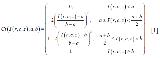
where I(r,c,z) represents the vBMD at a given voxel, and Ct(I(r,c,z);a,b) represents its membership to the class of cortical bone (from 0=no cortical bone to 1= cortical bone) given parameters a (a=mCt-2.5stdCt) and b (b=mCt+stdCt). This fuzzy s-shaped membership function was then used to perform a soft classification of the whole QCT scan based on vBMD values (Figure 2C). The membership values of this soft classification were then suitable for cortical bone thickness quantification using SIT. Thus for each vertex in the periosteal surface, cortical bone thickness was defined as the integral of membership values along streamlines starting at the periosteal surface, and ending at the endosteal surface (Figure 2D,E). Similar to the laminar analysis of magnetic resonance relaxation time values of knee cartilage described by Carballido-Gamio and Majumdar (42), each streamline was subdivided into n segments of equal length, which enabled the laminar encoding of vBMD values. The result of this step was a periosteal surface where each vertex was assigned a cortical bone thickness value and a vector of laminar cortical vBMD values.
Segmentation accuracy
One hundred thirty one scans were automatically segmented using the algorithm described above (the remaining scans were used to generate the MDT and the ten atlases). Qualitative assessment of the 131 segmentations was performed visually with overlays on a slice-by-slice basis in the axial orientation and coronal reformations, while quantitative validation of the accuracy of the segmentation algorithm was performed against manual segmentations of 80 scans: 50 scans from site A (mean ± std age =68±10 years; age range =47-89 years), and 30 scans from site B (mean ± std age =62±5 years; age range =54-69 years). Manual segmentations of the other 51 scans were not available. Validation was performed using three set agreement and three distance-based metrics. The three set agreement metrics were the dice similarity coefficient (DSC), the false negative rate (FNR), and the Jaccard index (JAC). The three distance-based metrics included the average symmetric distance (SYM) (43), the root-mean-square average symmetric distance (RMS-SYM) (43), and the modified Hausdorff distance (M-HAUS) (44).
DSC represents the size of the intersection of the gold standard and the automatic segmentations, divided by the average size of the two segmentations. Higher DSC indicates that the results match the gold standard better. A value of zero indicates no overlap between the segmentations, and a value of one indicates identical segmentations. The FNR measures the fraction of the gold-standard segmentation that was missed by the segmentation algorithm; therefore this metric must be small. JAC represents the size of the intersection of the gold standard and the automatic segmentations, divided by the size of the union of the two segmentations. If the segmentations have no common members JAC is zero; a value of one indicates that the segmentations are identical. As with DSC, a higher number indicates that the results match the gold standard better.
The average symmetric distance evaluates how close the voxels on the boundary of the automatic segmentation are to the voxels on the boundary of the gold standard segmentation, and vice versa. For each voxel on the boundary of the automatic segmentation, the Euclidean distance to the closest voxel on the boundary of the gold standard segmentation is computed and stored. The same process is applied from the boundary voxels of the gold standard segmentation to the boundary voxels of the automatic segmentation to provide symmetry. This metric is then defined as the average of all stored distances. A perfect segmentation would yield a value of zero millimeters. RMS-SYM is highly correlated with SYM, however, it penalizes large deviations from the true contour stronger. A value of zero millimeters also indicates a perfect segmentation. The M-HAUS is a shape similarity metric that has been previously used for template-based image matching. As with the SYM and RMS-SYM metrics, a value of zero millimeters indicates a perfect segmentation.
The equations defining both the set agreement and the distance-based metrics are listed in Table 1.

Full table
Multi-parametric precision
Reproducibility was assessed with root mean square coefficients of variation (CVRMS) and root mean square standard deviations for absolute errors (45). The precision of QCT-derived parameters based on automatic segmentations of the proximal femur was evaluated with 22 scan-rescan pairs with repositioning (site C; 8 pairs from manufacturer A; 14 pairs from manufacturer B). Three pairs had to be discarded due to scans with field-of-views excluding large portions of the inferior aspects of the femora. Subjects had a mean ± std age =69±5 years. QCT-derived parameters included: (I) compartmental vBMD; (II) compartmental tissue volume; (III) FEM bone strength; (IV) compartmental surface-based cortical bone thickness; (V) compartmental surface-based cortical bone vBMD; (VI) local surface-based cortical bone thickness; and (VII) local surface-based cortical bone vBMD. For the local assessments, the transformations computed to prescribe volumes of interest provided the alignment of the 22 pairs of scans to the MDT. Therefore cortical thicknesses and vBMD from each individual surface were mapped to the periosteal surface of the MDT at corresponding anatomic locations. For each vertex in the periosteal surface of the MDT, CVRMS and absolute precision errors were then computed. Vertex-wise paired t-tests were also performed to compare the 22 scan and rescan pairs of cortical bone thickness and cortical mean laminar vBMD maps. The resulting P values were corrected for multiple comparisons using false discovery rate (FDR) correction (q = 0.05) (46).
Results
Segmentation accuracy
Figure 1B,D,E show coronal cross-sections of partial results of a representative example of an automatic segmentation of the proximal femur. In these figures, the QCT being segmented has been color-coded in red, while the MDT was color-coded in cyan, thus the MDT remains fixed in the overlays. Figure 1B shows the result of applying the computed affine transformation to the QCT being segmented. Figure 1D shows the results of concatenating the affine transformation with each one of the three independent local affine transformations, while Figure 1E shows the concatenation of the affine transformation with the poly-affine registration (merging of Figure 1D using the fLEPT framework). The accuracy of the segmentation algorithm based on the three set agreement and three distance-based metrics is summarized in Table 2 indicating a mean DSC of 0.976±0.006 and a mean SYM of 0.203±0.057 mm. A total of ten QCT scans—out of 131—failed locally based on visual validation; all of them in the femoral head region (7.6%). Figure 3A shows representative automatic segmentations obtained in this study. In these figures, the automatically defined volumes of interest for the head, neck, and trochanter have been highlighted with different shades of red. A representative example of a failed segmentation is shown in Figure 3B.

Full table

Multi-parametric precision
Compartmental vBMD and compartmental tissue volume
Table 3 summarizes the reproducibility of compartmental vBMD and tissue volume parameters. The CVRMS for vBMD ranged from 0.89% for integral vBMD in the whole proximal femur, to 1.66% for trabecular vBMD in the femoral neck. All absolute precision errors were below 9 mg/cm3. The fact that the trabecular bone compartment in the femoral neck showed the lowest reproducibility was expected due to the rich marrow fat content in this region. With respect to bone volume, results were also as expected, with higher reproducibility for integral measurements, and lower reproducibility for thinner cortices. Nevertheless, CVRMS for all compartmental vBMD and bone volume measurements were better than 1.83%.

Full table
FEM bone strength
Table 4 summarizes the reproducibility of FEM bone strength for the nonlinear stance and nonlinear posterolateral fall configurations with CVRMS better than 3.6% and absolute precision errors below 342N.

Full table
Surface-based compartmental cortical bone parameters
Reproducibility results based on mean values of compartmental surface-based cortical bone thickness and mean laminar vBMD are summarized in Table 5 for the neck and trochanter together and individually. Although surface-based cortical bone parameters were also extracted for the femoral head, we decided not to include them due to the extremely thin cortices. Figure 2D shows a posterior view of a cortical bone thickness map calculated based on the length of the streamlines provided by the Laplace’s equation approach next to the SIT map (Figure 2E) for the same QCT scan. It is clear from this example that SIT incorporates partial volume effects into the computations. Scan-rescan examples for cortical SIT and mean laminar vBMD maps are shown in Figures 4 and 5, respectively.

Full table


Surface-based local cortical bone parameters
The local reproducibility of surface-based cortical bone thickness and mean laminar vBMD maps yielded the CVRMS and absolute precision error maps shown in Figures 6 and 7, respectively. As it was expected, higher reproducibility was observed for thick cortical bone regions like the inferior cortex. However, thinner regions such as the superior aspect of the femoral neck also showed high levels of reproducibility. The compartmental analysis of the CVRMS and absolute precision error maps shown in Figures 6 and 7 is summarized in Table 6.


Full table
The vertex-wise paired t-tests of spatially-normalized and smoothed (21,22) cortical bone thickness and mean laminar vBMD maps yielded nonsignificant vertices after FDR correction, thus indicating that the groups of scan and rescan cortical bone thickness and mean laminar vBMD maps were not significantly different from each other.
Discussion
QCT has become a leading imaging modality in osteoporosis research due to its 3D nature, its ability to distinguish between cortical and trabecular bone, and its use for multi-parametric assessments of bone quality. However, the starting point for all QCT analyses is a segmented hip, a procedure that is commonly accomplished in a semi-automated way and that requires several minutes of user interaction per clinical scan. Furthermore, previous QCT multi-parametric hip studies have been limited to a subset of the parameters investigated in this study. Here, we have presented an automatic framework to perform multi-parametric analyses of the proximal femur. This framework crops, segments, maps volumes of interest, and analyzes a QCT scan of the proximal femur in terms of vBMD, tissue volume, FEM bone strength, and cortical bone thickness. The accuracy of the segmentation algorithm was validated against manual segmentations, and the multi-parametric reproducibility evaluated based on scan-rescan acquisitions with repositioning. The QCT-derived parameters evaluated in this work are among the most widely studied quantitative outcome measures in osteoporosis research. Validation of the accuracy and evaluation of the reproducibility of the presented approaches was performed in a large dataset of QCT scans of older women from three clinical facilities and two different manufacturers yielding high fidelity to manual segmentations and CVRMS between 0.20-3.91% for all the parameters. The set of techniques and parameters presented in this work, along with those previously published by our group (20,23), enable comprehensive multi-parametric quantifications of the proximal femur in studies of etiology and osteoporosis treatment.
The three set agreement metrics and the three distance-based metrics listed in Tables 1,2, which were used to validate the accuracy of our segmentation approach, perform well compared to previous fully automatic hip QCT segmentation approaches. In the combined shape-intensity prior models work of Fritscher and colleagues (26), the authors reported a mean DSC of 0.992 and a mean Euclidean distance of 0.20 mm between the manually and automatically derived contours of scans with spatial resolution of 1.4×1.4×(0.6-5) mm3. However, the number of scans used to assess their reproducibility was quite small (n=10). In the model-guided demons work of Fritscher and colleagues (27) the authors used 47 QCT scans of the proximal femur to generate a SDM, and 21 QCT scans (gender and age were not reported) with isotropic spatial resolution (1.5 mm3) to test their algorithm under 120 different parameter configurations. The best overall mean configuration yielded an average Haussdorf distance (HAUS) and an average mean Euclidean distance of 3.38 mm and 0.76 mm, respectively. In the graph-cuts work of Krcah and colleagues an average HAUS of 5.4 mm was reported (28). Our mean DSC of 0.976, mean SYM of 0.203 mm, and mean M-HAUS of 0.253 mm (HAUS =3.928 mm) indicate the robustness of the proposed approach, especially considering that our validation was performed with 80 scans of older women from two different clinical sites and two highly anisotropic spatial resolutions (0.742×0.742×2.5 and 0.938×0.938×2.5 mm3).
The reproducibility of compartmental vBMD and compartmental bone volume (Table 3) was in agreement with previous reproducibility studies using scan-rescan acquisitions with repositioning. Using rigid registration and mutual information, Li and colleagues described a technique where the manually derived analyses of “baseline” scans were used to automatically quantify the “follow-up” acquisitions (47). The authors quantified the performance of their algorithm with 10 pairs of scans of postmenopausal women (mean ± std age =63±2 years) and observed an improvement with respect to pure manual quantification yielding CVRMS between 0.6-4.53% for compartmental vBMD, and 2.21-3.65% for compartmental tissue volume. The reproducibility of our automatic quantification of compartmental vBMD and compartmental tissue volume yielded CVRMS between 0.89-1.66% and between 0.20-1.82%, respectively. The observed improvement could be attributed to the cortical bone segmentation algorithm. While Li et al. utilized a 3D region growing approach solely based on voxel intensity values, a NL-FCM clustering algorithm using intensity and distance to the periosteal surface as segmentation features was used in this work.
Reproducible estimation of bone strength determined by QCT-based FEM is more challenging than the precision of vBMD and tissue volume. Variation in the boundaries of the proximal femur introduces sensitivity due to the inclusion/exclusion of cortical bone elements, which are heavily mechanically weighted because of their distance from the neutral axis and the fact that modulus varies with the square of vBMD. Furthermore, partial volume effects play a bigger role in critical regions such as the greater trochanter and the superior aspect of the femoral neck. Our reproducibility for whole bone strength calculated for the single-limb stance loading condition was slightly lower than that of Cody and colleagues (48). The authors reported a CVRMS of 1.85% based on ten pairs (eight women and two men) of scan-rescan acquisitions with repositioning (mean age =55.6 years), which were segmented based on a combination of manual drawing and thresholding operations. Our reproducibility was 3.51% and 3.59% for the nonlinear stance and nonlinear fall configurations (Table 4), respectively, for a population ~15 years older and more than double (n=22) the size of that of Cody et al. We believe that these numbers might be more representative of what could be achieved in the clinic, where detailed manual segmentations as those that can be obtained in a University setting are not viable. Regardless, the reproducibility achieved in this study should be sufficient to generate comparable results to those obtained based on manual segmentations. Using the same nonlinear FEM approach in the single-limb stance-loading configuration used here, Lang et al. reported a mean ~5-year reduction in bone strength of −451N (−4.2%) and −669N (−8.3%) in men (n=111; mean ± std age =77±6 years) and women (n=112; mean ± std age =77±5 years), respectively (49); while Keyak and colleagues reported a mean difference of 424N (11%) in bone strength between controls (n=97) and men with incident hip fracture (n=51) using the same nonlinear FEM approach in the posterolateral fall loading configuration used here (12). Furthermore, Keaveny et al. reported increases in bone strength in the order of 5.3% and 8.6% respectively after 12 and 36 months of treatment with denosumab once every 6 months for 36 months using nonlinear FEM in a configuration simulating a fall to the side of the hip (50).
Although cortical bone thickness derived from QCT scans has been utilized in numerous hip studies, especially in the femoral neck region, the reproducibility of this parameter has been reported few times. Kang and colleagues performed an intra- (3 times) and inter-operator (three observers) reproducibility study of vBMD, tissue volume, and cortical bone thickness of the femoral neck (same scan thus scanner instabilities and patient repositioning were not evaluated) in nine datasets (three women and six men; age range =33-73 years) with a spatial resolution of 0.3×0.3×1 mm3 (51). The authors reported CVRMS of 1.51% and 6.04% respectively for intra- and inter-operator reproducibility of cortical bone thickness in a spherical volume of interest. In a different intra-operator (3 times) reproducibility study of compartmental cortical bone thickness in the hip of 16 men, the authors reported CVRMS between 1.1% and 4.9% using QCT scans with a spatial resolution of 0.94×0.94×3 mm3 (10). Our compartmental analyses of surface-based cortical bone thickness using SIT (Table 5) yielded CVRMS values between 1.89% and 2.69%. Furthermore, our reproducibility analyses of cortical bone thickness did not require alignment of the “follow-up” to the “baseline” scans.
While the resistance of the proximal femur to fracture is dictated by its geometry, distribution of material properties, and magnitude and direction of the applied forces, it has been shown that the distribution of cortical bone plays a critical role (52,53). However, the local estimation of cortical bone thickness in the proximal femur is challenging due to the limited spatial resolution of the QCT systems. Recently, Treece and colleagues developed techniques to estimate local cortical bone thicknesses, cortical mass surface density, and the density of trabecular bone immediately adjacent to the cortex in the whole proximal femur using QCT (14,54,55). Unfortunately, scans with higher spatial resolution to generate gold standard 3D maps of cortical bone thickness and vBMD to quantify the accuracy of our technique were not available. However, the CVRMS and absolute precision error maps shown in Figures 6 and 7, and the compartmental mean values of the local analyses listed in Table 6 show high levels of local reproducibility (<4%) and small absolute precision errors. Nevertheless, our results indicate that studies such as those of Poole and colleagues (21,22) are feasible with our cortical bone thickness quantification technique. In a study of osteoporosis treatment, significant local cortical bone thickening of ~4% or more was reported after 24 months of recombinant human PTH [hPTH-(1-34)] (119 femora from 65 women) (21); while in a cross-sectional study of hip fracture, significant local cortical bone thickness differences of at least ~15% and ~10% were observed between controls (n=75) and women with neck (n=36) and trochanteric (n=39) hip fractures, respectively (22).
In conclusion, in this study we have presented an automatic framework to perform accurate and precise multi-parametric assessments of the proximal femur using QCT imaging. The set of QCT parameters that were evaluated included those most studied in osteoporosis research. Our subjects were typical of the elderly female population of interest, with scans obtained across multiple clinical sites and manufacturers, thus representing the conditions involved in clinical trials and other large-scale multi-center studies.
Appendix A
Merging of the three affine registrations was done within the fast Log-Euclidean poly-affine framework (fLEPT) with Gaussian weighted maps for the regions shown in Figure 1C, thus yielding stationary velocity fields (SVFs):
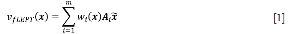
In Eq. [1], x is a 3×1 vector,  is a 4×1 vector, m is the number of regions (m=3), wi (x) are normalized weights for region
 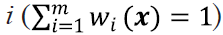 , and Ai is a 3×4 matrix obtained in the following way:
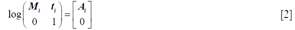
where log stands for the principal matrix logarithm, Mi is a 3×3 matrix with the linear part of an affine transformation, and ti is a 3×1 vector with the translation component. As proposed by Arsigny and colleagues, the exponential exp(V) of a smooth velocity field V(x) defines the flow at time 1 of the stationary ordinary differential equation  . Thus the deformation can be computed within the SVF framework for diffeomorphisms by recursively using the scaling and squaring method, i.e.,
  , where N is large enough so that
  is close enough to zero. Intuitively this means that the deformations at time 1 can be computed by recursively composing 2N times the very small deformations observed at time
  .
.
Appendix B
The NL-FCM algorithm minimizes the following energy function:
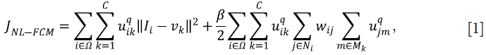
In Eq. [1], uik represents the membership of the ith voxel to the kth class; C represents the number of classes;  ; q controls the level of fuzziness of the segmentation (if q gets close to 1, the segmentation gets close to a hard segmentation); Ii represents the grey-level of the ith voxel in the image domain Ω; vk represents the centroid of the kth class; β controls the trade-off between the data-term and the NL regularization term; Ni is the set of neighbors of the ith voxel; Mk={1,…,C}\{k}; and the weight for the ith and jth voxels wij is defined as:
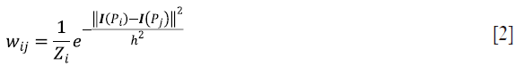
In Eq. [2], Zi is a normalization constant, h is a smoothing parameter, and the distance between patches is computed as follows:
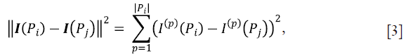
where I(Pi) is the vector containing the grey-levels of the ith patch, and I(p)(Pi) is the pth element of this vector. Intuitively, if patches I(Pi) and I(Pj) are similar, there might belong to the same tissue thus increasing wij, and consequently the influence of the NL regularization term in Eq. [1]. Conversely, if two patches are quite different, their weight should decrease, thus reducing the influence of the NL regularization term, since there is a lower probability that the jth voxel might have a good influence on the classification of the current ith voxel.
Acknowledgements
Funding: This work was supported by the NIH/NIAMS under grants R01AR064140, R01AR060700, R01AR054496 and P30AR066262, and by the Intramural Research Program of the NIH, National Institute on Aging, under the contract HHSN311200900345P.
Footnote
Conflicts of Interest: The authors have no conflicts of interest to declare.
References
- Budhia S, Mikyas Y, Tang M, Badamgarav E. Osteoporotic fractures: a systematic review of U.S. healthcare costs and resource utilization. Pharmacoeconomics 2012;30:147-70. [PubMed]
- Roy A, Heckman MG, O'Connor MI. Optimizing screening for osteoporosis in patients with fragility hip fracture. Clin Orthop Relat Res 2011;469:1925-30. [PubMed]
- Burge R, Dawson-Hughes B, Solomon DH, Wong JB, King A, Tosteson A. Incidence and economic burden of osteoporosis-related fractures in the United States, 2005-2025. J Bone Miner Res 2007;22:465-75. [PubMed]
- Blake GM, Fogelman I. The role of DXA bone density scans in the diagnosis and treatment of osteoporosis. Postgrad Med J 2007;83:509-17. [PubMed]
- Genant HK, Engelke K, Prevrhal S. Advanced CT bone imaging in osteoporosis. Rheumatology (Oxford) 2008;47 Suppl 4:iv9-16. [PubMed]
- Sundquist J, Winkleby MA, Pudaric S. Cardiovascular disease risk factors among older black, Mexican-American, and white women and men: an analysis of NHANES III, 1988-1994. Third National Health and Nutrition Examination Survey. J Am Geriatr Soc 2001;49:109-16. [PubMed]
- Lian KC, Lang TF, Keyak JH, Modin GW, Rehman Q, Do L, Lane NE. Differences in hip quantitative computed tomography (QCT) measurements of bone mineral density and bone strength between glucocorticoid-treated and glucocorticoid-naive postmenopausal women. Osteoporos Int 2005;16:642-50. [PubMed]
- Schuit SC, van der Klift M, Weel AE, de Laet CE, Burger H, Seeman E, Hofman A, Uitterlinden AG, van Leeuwen JP, Pols HA. Fracture incidence and association with bone mineral density in elderly men and women: the Rotterdam Study. Bone 2004;34:195-202. [PubMed]
- Lang T, LeBlanc A, Evans H, Lu Y, Genant H, Yu A. Cortical and trabecular bone mineral loss from the spine and hip in long-duration spaceflight. J Bone Miner Res 2004;19:1006-12. [PubMed]
- Yang L, Burton AC, Bradburn M, Nielson CM, Orwoll ES, Eastell R. Osteoporotic Fractures in Men (MrOS) Study Group. Distribution of bone density in the proximal femur and its association with hip fracture risk in older men: the osteoporotic fractures in men (MrOS) study. J Bone Miner Res 2012;27:2314-24. [PubMed]
- Genant HK, Libanati C, Engelke K, Zanchetta JR, Høiseth A, Yuen CK, Stonkus S, Bolognese MA, Franek E, Fuerst T, Radcliffe HS, McClung MR. Improvements in hip trabecular, subcortical, and cortical density and mass in postmenopausal women with osteoporosis treated with denosumab. Bone 2013;56:482-8. [PubMed]
- Keyak JH, Sigurdsson S, Karlsdottir GS, Oskarsdottir D, Sigmarsdottir A, Kornak J, Harris TB, Sigurdsson G, Jonsson BY, Siggeirsdottir K, Eiriksdottir G, Gudnason V, Lang TF. Effect of finite element model loading condition on fracture risk assessment in men and women: the AGES-Reykjavik study. Bone 2013;57:18-29. [PubMed]
- Kopperdahl DL, Aspelund T, Hoffmann PF, Sigurdsson S, Siggeirsdottir K, Harris TB, Gudnason V, Keaveny TM. Assessment of incident spine and hip fractures in women and men using finite element analysis of CT scans. J Bone Miner Res 2014;29:570-80. [PubMed]
- Treece GM, Gee AH, Mayhew PM, Poole KE. High resolution cortical bone thickness measurement from clinical CT data. Med Image Anal 2010;14:276-90. [PubMed]
- Johannesdottir F, Poole KE, Reeve J, Siggeirsdottir K, Aspelund T, Mogensen B, Jonsson BY, Sigurdsson S, Harris TB, Gudnason VG, Sigurdsson G. Distribution of cortical bone in the femoral neck and hip fracture: a prospective case-control analysis of 143 incident hip fractures; the AGES-REYKJAVIK Study. Bone 2011;48:1268-76. [PubMed]
- Carpenter RD, Sigurdsson S, Zhao S, Lu Y, Eiriksdottir G, Sigurdsson G, Jonsson BY, Prevrhal S, Harris TB, Siggeirsdottir K, Guðnason V, Lang TF. Effects of age and sex on the strength and cortical thickness of the femoral neck. Bone 2011;48:741-7. [PubMed]
- Carballido-Gamio J, Nicolella DP. Computational anatomy in the study of bone structure. Curr Osteoporos Rep 2013;11:237-45. [PubMed]
- Li W, Kezele I, Collins DL, Zijdenbos A, Keyak J, Kornak J, Koyama A, Saeed I, Leblanc A, Harris T, Lu Y, Lang T. Voxel-based modeling and quantification of the proximal femur using inter-subject registration of quantitative CT images. Bone 2007;41:888-95. [PubMed]
- Li W, Kornak J, Harris T, Keyak J, Li C, Lu Y, Cheng X, Lang T. Identify fracture-critical regions inside the proximal femur using statistical parametric mapping. Bone 2009;44:596-602. [PubMed]
- Carballido-Gamio J, Harnish R, Saeed I, Streeper T, Sigurdsson S, Amin S, Atkinson EJ, Therneau TM, Siggeirsdottir K, Cheng X, Melton LJ 3rd, Keyak J, Gudnason V, Khosla S, Harris TB, Lang TF. Proximal femoral density distribution and structure in relation to age and hip fracture risk in women. J Bone Miner Res 2013;28:537-46. [PubMed]
- Poole KE, Treece GM, Ridgway GR, Mayhew PM, Borggrefe J, Gee AH. Targeted regeneration of bone in the osteoporotic human femur. PLoS One 2011;6:e16190. [PubMed]
- Poole KE, Treece GM, Mayhew PM, Vaculík J, Dungl P, Horák M, Štěpán JJ, Gee AH. Cortical thickness mapping to identify focal osteoporosis in patients with hip fracture. PLoS One 2012;7:e38466. [PubMed]
- Carballido-Gamio J, Harnish R, Saeed I, Streeper T, Sigurdsson S, Amin S, Atkinson EJ, Therneau TM, Siggeirsdottir K, Cheng X, Melton LJ 3rd, Keyak JH, Gudnason V, Khosla S, Harris TB, Lang TF. Structural patterns of the proximal femur in relation to age and hip fracture risk in women. Bone 2013;57:290-9. [PubMed]
- Bredbenner TL, Mason RL, Havill LM, Orwoll ES, Nicolella DP. Osteoporotic Fractures in Men (MrOS) Study. Fracture risk predictions based on statistical shape and density modeling of the proximal femur. J Bone Miner Res 2014;29:2090-100. [PubMed]
- Kang Y, Engelke K, Kalender WA. A new accurate and precise 3-D segmentation method for skeletal structures in volumetric CT data. IEEE Trans Med Imaging 2003;22:586-98. [PubMed]
- Fritscher KD. Grünerbl A, Schubert R. 3D image segmentation using combined shape-intensity prior models. Int J CARS 2007;1:341-50.
- Fritscher KD, Schuler B, Roth T, Kammerlander C, Blauth M, Schubert R. Model guided diffeomorphic demons for atlas based segmentation. Proc of SPIE: Medical Imaging 2010.
- Krcah M, Székely G, Blanc B. Fully automatic and fast segmentation of the femur bone from 3D-CT images with no shape prior. Proc of IEEE ISBI 2011.
- Arsigny V, Pennec X, Ayache N. Polyrigid and polyaffine transformations: a novel geometrical tool to deal with non-rigid deformations - application to the registration of histological slices. Med Image Anal 2005;9:507-23. [PubMed]
- Arsigny V, Commowick O, Ayache N, Pennec X. A Fast and Log-Euclidean Polyaffine Framework for Locally Linear Registration. J Math Imaging Vis 2009;33:222-38.
- Keyak JH. Improved prediction of proximal femoral fracture load using nonlinear finite element models. Med Eng Phys 2001;23:165-73. [PubMed]
- Keyak JH, Kaneko TS, Tehranzadeh J, Skinner HB. Predicting proximal femoral strength using structural engineering models. Clin Orthop Relat Res 2005;(437):219-28. [PubMed]
- Aganj I, Sapiro G, Parikshak N, Madsen SK, Thompson PM. Measurement of cortical thickness from MRI by minimum line integrals on soft-classified tissue. Hum Brain Mapp 2009;30:3188-99. [PubMed]
- Jones SE, Buchbinder BR, Aharon I. Three-dimensional mapping of cortical thickness using Laplace's equation. Hum Brain Mapp 2000;11:12-32. [PubMed]
- Vercauteren T, Pennec X, Perchant A, Ayache N. Non-parametric diffeomorphic image registration with the demons algorithm. Med Image Comput Comput Assist Interv 2007;10:319-26. [PubMed]
- Cachier P, Pennec X. 3D non-rigid registration by gradient descent on a Gaussian-windowed similarity measure using convolutions. Hilton Head Island South Carolina Usa IEEE Computer Society 2000:182-9.
- Heckemann RA, Hajnal JV, Aljabar P, Rueckert D, Hammers A. Automatic anatomical brain MRI segmentation combining label propagation and decision fusion. Neuroimage 2006;33:115-26. [PubMed]
- Vercauteren T, Pennec X, Perchant A, Ayache N. Symmetric log-domain diffeomorphic Registration: a demons-based approach. Med Image Comput Comput Assist Interv 2008;11:754-61. [PubMed]
- Caldairou B, Rousseau F, Passat N, Habas P, Studholme C, Heinrich C. A Non-Local Fuzzy Segmentation Method: Application to Brain MRI. Lect Notes Comput Sc 2009;5702:606-13.
- Borggrefe J, Graeff C, Nickelsen TN, Marin F, Glüer CC. Quantitative computed tomographic assessment of the effects of 24 months of teriparatide treatment on 3D femoral neck bone distribution, geometry, and bone strength: results from the EUROFORS study. J Bone Miner Res 2010;25:472-81. [PubMed]
- Acosta O, Bourgeat P, Zuluaga MA, Fripp J, Salvado O, Ourselin S. Alzheimer's Disease Neuroimaging Initiative. Automated voxel-based 3D cortical thickness measurement in a combined Lagrangian-Eulerian PDE approach using partial volume maps. Med Image Anal 2009;13:730-43. [PubMed]
- Carballido-Gamio J, Majumdar S. Atlas-based knee cartilage assessment. Magn Reson Med 2011;66:574-83. [PubMed]
- Heimann T, van Ginneken B, Styner MA, Arzhaeva Y, Aurich V, Bauer C, Beck A, Becker C, Beichel R, Bekes G, Bello F, Binnig G, Bischof H, Bornik A, Cashman PM, Chi Y, Cordova A, Dawant BM, Fidrich M, Furst JD, Furukawa D, Grenacher L, Hornegger J, Kainmüller D, Kitney RI, Kobatake H, Lamecker H, Lange T, Lee J, Lennon B, Li R, Li S, Meinzer HP, Nemeth G, Raicu DS, Rau AM, van Rikxoort EM, Rousson M, Rusko L, Saddi KA, Schmidt G, Seghers D, Shimizu A, Slagmolen P, Sorantin E, Soza G, Susomboon R, Waite JM, Wimmer A, Wolf I. Comparison and evaluation of methods for liver segmentation from CT datasets. IEEE Trans Med Imaging 2009;28:1251-65. [PubMed]
- Dubuisson MP, Jain AK. A Modified Hausdorff Distance for Object Matching. Int C Patt Recog 1994:566-8.
- Glüer CC, Blake G, Lu Y, Blunt BA, Jergas M, Genant HK. Accurate assessment of precision errors: how to measure the reproducibility of bone densitometry techniques. Osteoporos Int 1995;5:262-70. [PubMed]
- Genovese CR, Lazar NA, Nichols T. Thresholding of statistical maps in functional neuroimaging using the false discovery rate. Neuroimage 2002;15:870-8. [PubMed]
- Li W, Sode M, Saeed I, Lang T. Automated registration of hip and spine for longitudinal QCT studies: integration with 3D densitometric and structural analysis. Bone 2006;38:273-9. [PubMed]
- Cody DD, Hou FJ, Divine GW, Fyhrie DP. Short term in vivo precision of proximal femoral finite element modeling. Ann Biomed Eng 2000;28:408-14. [PubMed]
- Lang TF, Sigurdsson S, Karlsdottir G, Oskarsdottir D, Sigmarsdottir A, Chengshi J, Kornak J, Harris TB, Sigurdsson G, Jonsson BY, Siggeirsdottir K, Eiriksdottir G, Gudnason V, Keyak JH. Age-related loss of proximal femoral strength in elderly men and women: the Age Gene/Environment Susceptibility Study--Reykjavik. Bone 2012;50:743-8. [PubMed]
- Keaveny TM, McClung MR, Genant HK, Zanchetta JR, Kendler D, Brown JP, Goemaere S, Recknor C, Brandi ML, Eastell R, Kopperdahl DL, Engelke K, Fuerst T, Radcliffe HS, Libanati C. Femoral and vertebral strength improvements in postmenopausal women with osteoporosis treated with denosumab. J Bone Miner Res 2014;29:158-65. [PubMed]
- Kang Y, Engelke K, Fuchs C, Kalender WA. An anatomic coordinate system of the femoral neck for highly reproducible BMD measurements using 3D QCT. Comput Med Imaging Graph 2005;29:533-41. [PubMed]
- Carpenter RD, Beaupré GS, Lang TF, Orwoll ES, Carter DR. Osteoporotic Fractures in Men (MrOS) Study Group. New QCT analysis approach shows the importance of fall orientation on femoral neck strength. J Bone Miner Res 2005;20:1533-42. [PubMed]
- Mayhew PM, Thomas CD, Clement JG, Loveridge N, Beck TJ, Bonfield W, Burgoyne CJ, Reeve J. Relation between age, femoral neck cortical stability, and hip fracture risk. Lancet 2005;366:129-35. [PubMed]
- Treece GM, Poole KE, Gee AH. Imaging the femoral cortex: thickness, density and mass from clinical CT. Med Image Anal 2012;16:952-65. [PubMed]
- Treece GM, Gee AH. Independent measurement of femoral cortical thickness and cortical bone density using clinical CT. Med Image Anal 2015;20:249-64. [PubMed]

