
A theory of fine structure image models with an application to detection and classification of dementia
Introduction
When viewing a complete, as opposed to a region of interest, medical image such as an axial MRI brain scan, the diagnostician typically makes an overall image assessment and then studies from region to region seeking elements of normal structure and pathology. The eye cannot readily assess the thousands of small image regions for comparison. Thus, image fine structure information at the individual pixel level, of necessity, has been visually ignored. Whether such fine structure of closely spaced pixels, of any size image, will be useful for medical purposes is an open question since it has been difficult to obtain such data. Further, in the problem of diagnosing neurological diseases, our bioengineering application addresses a long recognized clinical need of dementia diagnosis: MR image quantification has been, and still is, an arduous task, currently requiring considerable processing time and operator attention (1). In Alzheimer’s disease (AD), for example, it is difficult to distinguish normal aging changes of increased ventricular and sulcus size from AD degeneration.
The definitive diagnosis of dementia is by autopsy but of the ten recognized cognitive tests, the most popular in use is the Mini Mental State Examination (MMSE) which has the best correlation with autopsy outcomes and is the most useful in following diagnosed dementia over time (2). Therefore we use subject MMSE scores to categorize normal or demented subjects. To support this definition of subject cognitive state, we seek a brain scan image model whose parameters not only capture discriminating image information but also indicate which parameters of the image carry the most discriminating information as measured by their inferred confidence intervals (3).
Materials and methods
Our original computational method is based on ordinary least squares (OLS) regression because we discovered a simple matrix transformation that enables images to be represented as linear combinations of row and column spatial lags of the original image. These row and column lagged images give rise to the “fine structure” description of the images we model because the row and column spatially lagged images are visually indistinct from the original. The key step in our analysis is to transform any two dimensional (2D) image pixel array to a one dimensional (1D) pixel array. Next we show that transformed images can be modeled by traditional OLS methods. Therefore, under verified distributional conditions, the OLS model parameters can be tested for statistical significance. This is an important model property as it means recognized neurological conditions can be tested for causality by parameter significance. In addition, the most significant parameters carry the most discrimination information in implementing image classifications.
Image model development
To reduce a 2D pixel array (an image) to a 1D pixel array (a column) a transformation called vectorization is applied by stacking the left-most column of image pixels onto its neighbor pixel column and these two columns onto the third and so on, until all pixel columns are stacked (4). For example, an image A of 208 rows and 176 columns of pixels becomes a single column of [208] × [176]=36,608 pixels. We call this column the vectorized form of A and write it as vec(A). The next step is to recognize that any image y(i,j), whose intensity y at pixel location (i,j), can be hypothesized to be a solution of the linear autoregressive (AR) model (5).
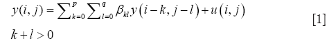
In Eq. [1], u(i,j) is a random process error term and we note Eq. [1] is a discrete approximation to a general, linear, causal, partial differential equation in two space dimensions.
The final step is to show, see Appendix A1, that if ct and At are real constants and matrices then:

Define yo = vec[y(i,j)], x1 = vec[y(i,j-1)], x2 = vec[y(i-1,j)], .., xp+q+qp = vec[y(i-p,j-q)], and uo = vec[u(i,j)]. By Eq. [2], the model in Eq. [1], with β as a column vector with p+q+qp elements βkl, has the familiar OLS regression form.

In Eq. [3], Xβ is called a minimum variance representation (MVR) of the vectorized image yo if a β can be found such that uoT uo is minimized. A necessary and sufficient condition that such a β exists is:
MVR existence theorem: [Th1].
An image of pixel intensity y(i,j) has a MVR in the form of

if and only if k+l>0, the image column vectors x1x2 .. xp +q +pq are linearly independent.
When this condition is met the minimizing β satisfies:

and the image MVR is:

The finite sample form of Eq. [3] employed to estimate β is

where b is the OLS estimate of the population (true) value β and the vector eo estimates the random residual vector uo. Using the format of Eq. [6], each image of the Alzheimer’s Disease Neuroimaging Initiative (ADNI) and Open Access Series of Imaging Studies (OASIS) data sets had an estimated MVR, denoted as Xb, minimizing eoTeo and computed as:
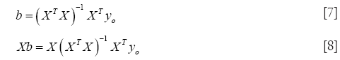
The integer p, q orders are determined by increasing p and q so that (XTX)−1 exists for all image data. For both the ADNI and OASIS data this was for p=q=2. Larger p or q made (XTX) ill-conditioned. If the image to be modeled is m by n pixels then the minimum variance realization Xb of the image is a column vector of (m-p) × (n-q) by 1 pixels. To realize the 2D picture of Xb it must be unstacked into 2D image model starting at the top of Xb.
Only in the rarest of cases will the residual vector eo in Eq. [6] test to be white Gaussian noise which would permit Student’s t-tests of parameter statistical significance. So we have developed, see Appendix A2, a nonparametric significance statistic, wkl, based on the Chebychev inequality (6). |wkl| measures the width, normalized by bkl, of a 1-α confidence interval of the true βkl. The smaller |wkl| is for a given bkl, the more significant is the estimated parameter bkl multiplying lagged image vec[y(i-k,j-l)]. For the diagnostician the confidence interval of βkl is the most important property derived from its estimate bkl since it tells him the probability with which the true parameter he seeks, βkl, is estimated by what he estimates, bkl.
The X matrix in Eq. [6] has eight column vectors, eight spatially lagged, vectorized images of y(i-k,j-l) for k =0,1,2, l =0,1,2, k + l >0. However, we found that adding a column of ones to X to account for image sample means slightly increases the likelihood of correct classification as developed in the following section. Relative to the theoretical model in Eq. [1], this amounts to adding a constant to the right-hand side. The column of ones is crucial because it assures the residual vector eo in Eq. [6] and is estimated without bias, a bias which would also induce a bias in the estimated vector b.
Optimal image classification
In this section we derive a discriminator by which a given subject’s MMSE score identifies the subject as normal or demented and also gives a ranking statistic to compare with other subjects in the same class. A range of MMSE scores is chosen and subjects with scores in that range are categorized as members of the demented class. Another unique MMSE range is chosen for those subjects categorized as normal subjects. Let Nd and Nn be the respective number of subjects in each class. For each subject Eq. [7] estimates a b vector of size p+q+pq+1=9. These are arranged in parameter matrices Bd, 9 by Nd and Bn, 9 by Nn and the pooled parameter matrix Bp which is 9 by Nd + Nn. Let  be estimates of the covariance matrices of Bd, Bn, and Bp. The projections onto the scalar z axis of zn = Bnv, zd = Bdv, and zp = Bpv are maximally separated in sample means if the projection vector v satisfies the Fisher linear discriminant eigenvector identity (7),

for the only nonzero eigenvalue γ1. In Eq. [9], n1 = Nd + Nn –1, n2 = Nn –1, n3 = Nd –1. For even modest sample sizes, Nd and Nn ≥10, a Kolmogorov-Smirnov test (K-S test) confirms the hypothesis the z projections are normally distributed (8).
Since zn and zd are normally distributed with estimated densities fn(z) and fd(z), the Kullback-Leibler discrimination (KLD) statistic for a zero threshold, Lo(z), is a convenient means of comparing projections for “strength of class membership” since |Lo(z)| is monotonic with membership probability (9).
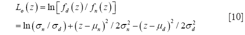
In Eq. [10], means and variances are estimated from the sample z projections. Lo(z) >0 classifies a z-projection as demented and Lo(z) <0 as a normal.
The KLD statistics provide a graphical display of TP, TN, FP, and FN measures of the classification algorithm.
Large-sample ADNI dataset
Our large sample study employed ADNI archive axial MR image slices. The images were 1.5 T, T1 weighted using the MP Rage sequence, calibration scans for B1 correction, dual fast spin echo and were 256 by 170 gray scale pixels. All ADNI images were selected from one slice axially above the anterior commissure brain structure. ADNI subject inclusion criteria varied over four classes: (I) normal subjects had no subjective memory complaints; (II) normal memory function stratified by educational attainment; (III) MMSE scores between 24 and 30; and (IV) a Clinical Dementia Rating (CDR) of 0. EMCI subjects had subjective memory complaints, abnormal memory function stratified by age, MMSE 24 to 30, a CDR of 0.5, and AD could not be diagnosed at time of screening visit. LMCI subjects had the same criteria as the EMCI subjects but educational attainment was lower. AD subjects had memory complaints, abnormal memory function, MMSE scores 20 to 27, CDR of 0.5 to 1.0, and satisfied a NINCDS criteria for probable AD. The 50 subjects we took as normal were screened as males, ages 65 to 84 years with MMSE scores of 29 to 30. The 47 subjects we took as demented were of ages 65 to 84 years with MMSE scores of 17 to 27. Therefore the 97 subjects were identified as normal or demented according to the range of their MMSE scores. The 97 subjects so identified exhausted the four classes cited above for the constraints we specified. It is likely that about 70% of the categorized demented subjects suffered from AD (10). The chosen MMSE score ranges are typical for normal/demented studies with 20 year age spans (2). All ADNI axial images had cranium and dura artifacts manually cropped. Figure 1 displays typical ADNI images.

Small-sample OASIS data set
Our small sample study employed OASIS axial MR image slices screened as right-handed males of ages 65 to 75 years with MMSE scores of 29 to 30. The database produced 14 such images we refer to as the normal class. Screening for right-handed males of ages 67 to 84 years with MMSE scores of 17 to 27 produced 12 images we refer to as the demented class. These images came from a set of 416 subjects aged 18 to 96. For each subject, 3 or 4 individual T1-weighted MRI scans obtained in single scan sessions were averaged to get the images, 208 by 176 pixels, for our study. A total of 100 of the included subjects over the age of 60 had been clinically diagnosed with very mild to moderate AD, in addition, a reliability data set of 20 non-demented subjects imaged on a subsequent visit within 90 days of their initial session were available as normal subjects. OASIS images had dura and cranium artifacts manually cropped. All axial images from the OASIS archive were at a fixed, unspecified number of 1.5 mm slices from the anterior commissure brain structure. Figure 2 are typical OASIS images.

Results
Typical image OLS models, parameters, and statistics
All 123 images were modeled using the OLS Eqs. [7] and [8] and the |wkl| significance statistics (for a 95% confidence interval) computed for all bkl parameters. Figure 3 is a typical OLS scatter diagram, this for a demented subject from the OASIS dataset. The regression R2 for this model is typical of image regressions for both datasets as they all exceeded 99%. Figure 4 illustrates typical estimation results for two OASIS subjects and Table 1 lists the OLS bkl parameters and |wkl| statistics for the images in Figure 4. Typical normal and demented images and models of ADNI subjects are shown in Figure 5; bkl parameters and |wkl| statistics for these two ADNI subjects are in Table 4.


Full table


Full table

Full table

Full table
Sample means of model parameters and their significance statistics
Table 3 tabulates sample means of estimated parameters and sample means of their |wkl| statistics for the OASIS dataset and Table 2 tabulates these sample means for the ADNI dataset. With sample sizes of 50 and 47, the entrees in Table 2 are highly significant. For example, an interpretation of the mean(|wkl|) value of b01 is: with a probability of 0.95 the average true demented parameter β01 is in the interval 1.0812±0.0232; for normal subject b01 the 95% interval of β01 is 1.1174±0.0228.
Table 3 entrees for the OASIS (26 samples) dataset do not differ dramatically from the ADNI Table 2 entrees but there is a subtle shift of the most significant bkl parameter from b10 for the OASIS data to b01 for the ADNI data. This shift is interpreted later.
Optimal image classification
Figure 6 shows the inferred probability density functions of the ADNI z-projections resulting from projecting the bkl parameters with the eigenvector solution of Eq. [9]. These probability densities passed K-S tests for normality at level 10−5 which decisively supports the classification probability inference of the KLD statistics, computed from Eq. [10] and also shown in Figure 6. Figure 7 shows the inferred z-projection probability density functions for the OASIS subjects. These densities passed K-S tests for normality at level 10−3. An interpretation of the KLD statistics for the demented (normal) projections is that the larger (smaller) the KLD statistic is, then the more likely the sample is correctly classified. For example, in Figure 7 the leftmost z-projection (near 114.4) corresponds to demented sample number 7 with KLD of 20. On the other hand, the demented projection near 115.4 corresponds to sample number 2 which has a negative KLD and this sample is misclassified.


We also performed a cross validation test for the ADNI images by randomly selecting 12 normal and 12 demented subjects to be test subjects for a training classifier based on 38 normal and 35 demented subjects. The results of that test are shown in Figure 8. In that figure the accuracy of the training classifier (inferred z-projection densities shown) was 69/73=94.5%, while the test subjects were classified with an accuracy of 22/24=91.7%.

Comparison with other medical image classifiers
The first comparison study is selected because it is comprehensive in feature extractions (gray level histogram, gray level co-occurrence matrix, shape invariant moment, and FFT frequency), uses an average of 408 CT and MR images (102 testing for a 25% testing-to-training ratio) and tests 4 popular classification methods (C4.5, SVM, naive Bayes, KNN) (11). The averages over feature extractions shown in Table 5 are to be compared to our OLS method’s 91.7% accuracy using a 24.2% testing-to-training ratio. The authors give no computational time or computer specification results.

Full table
The second comparison study is selected because it tests an advanced form of the random forest (RF) classifier, uses a test–to-training ratio of 33% on 300 region of interest MR images of 256×216 pixels each (12). They report a computation time of 304 seconds average with 86.4% accuracy using a 2.66 GHz machine of unspecified RAM.
The final comparison study is selected because it tests three forms of the RF classifier, uses 10 fold cross-validation, and gives comprehensive computation times using a 3.4 GHz, 12 GB RAM computer (13). Images are 3 color of 174 colon biopsies. The grid size modeled is a rather crude 49 blocks. The original feature set produced an accuracy of 91.3% averaged over the three classifiers. Increasing features from 20 to 50 boosted the average accuracy to 93.0% with run times of 104 seconds averaged over the three RF classifiers. The authors quote five other comparable colon studies whose average accuracy is 85.43%.
The dramatic difference between our OLS method and those cited above is computation time. Using a 3.00 GHz computer with 3.72 RAM our all-training result, Figure 6, required 0.9014 seconds, Figure 7 took 0.2516 seconds while Figure 8 required 0.6466 seconds. The RF classifier of ROI images (of a comparable number of pixels) cited above required 224 seconds on a machine 13% slower than ours. Derating 224 seconds by 13% and increasing our run time by 300/73 to compensate for sample sizes implies our runtime is 195/2.66=73.3 times faster than the cited classification of ROI images.
The colon biopsy classifiers must classify red, green and blue images so we must triple our runtimes and compensate for sample sizes by 174/73. This gives our estimated comparable runtime of 0.6466×3×2.38=4.62 seconds which is 104/4.62=22.5 times faster than the RF image classifiers. Individually, the red, green and blue images required 34, 48, and 22 seconds respectively. OLS equivalent time is 2.38×0.6466=1.54 seconds for each color.
Summary
Including the 5 colon studies cited in (13), we have compared our OLS classifier to 13 classifiers from the literature and our training-test accuracy of 91.7% is better than all but one average.
In the runtime domain, none of the cited classifiers is competitive with the OLS classifier. The lowest runtime cited for the reviewed classifiers is a minimum of 14 times slower than the OLS classifier.
The implied superiority of the OLS method over the comparison image classification methods in accuracy and computation times results from two properties of the OLS method: (I) the OLS image models are rigorously defined in terms of statistical estimation of partial difference equation solutions; (II) the vec(.) transformation and its theoretical preservation of the OLS format for the partial difference equation model and [Th1], is complemented by a runtime-optimized vec(.) function on Matlab.
Discussion
The innovation of OLS image modeling
Modeling of discrete time series, representing native discrete time systems or discretized ordinary differential equations, has advanced to the stage that transfer function theory and ubiquitous software to model data are commonplace (14-16). OLS is the estimation method of choice for such linear system models (also called 1D system because they employ one independent variable). In our past work we have found the estimated parameters of such models are capable of classifying the subject data they model and can provide insight into physical system interpretations (17-21).
The AR model hypothesis in Eq. [1], the vector transformation in Eq. [2], and the MVR theorem [Th1] make available to 2D modeling all of the methods cited above for 1D systems. Further, images are a special case of 2D systems which include image modalities of X-ray, US, MRI, PET, and SPECT.
Interpretation of image model parameters for large brain scans
While OLS models of medical image parameters are capable of robust image classification, an equally important utility lies in their diagnostic potential.
Diagnosis is taken to be at two image sizes: (I) entire brain scans, for example the axial brain scans of this study; (II) and ROI size images which are not investigated in this study. An interpretation of average image parameters we found in image height to width ratios. This ratio calculated for all ADNI and OASIS images averages 24.9% greater for the ADNI images. Thus, the subtle shift, noted above, in the most significant parameters b10 in Table 3 to b01 in Table 2 is due to the ADNI images having more informative pixel columns than rows, thereby favoring correlations between y(i,j) and y(i,j-1) as measured by b01. Analogously, b10, relating y(i,j) and y(i-1,j), is more significant for the OASIS images whose pixel rows are more informative than their columns.
Image parameter medical interpretation addresses the difficulty in distinguishing which of seven possible dementia types a given subject is suffering. Having nine parameter image models and statistics to measure individual parameter significance presents the opportunity to design a study in which cognitive test scores and post mortem dementia identification outcomes can be used to identify parameters or groups of parameters specific to dementia types.
Figures 1,2 and 4,5 indicate a large within-sample variation in ventricle size as a percent of total brain scan. To determine the possible classifying effect this variation might have on z-projections, a 20% image random sample from both datasets was used to cross-correlate ventricle area with z-projection size. The correlations were not significant at the 10% level. Further, even within-class correlation was not evident, two OASIS demented subjects differed 67% in ventricle area and only 2.2×10⁻⁴ percent in z-projection size. The reason for this outcome lies in the observation that ventricles are interpreted by OLS as zero pixel intensity background similar to that which fills the rectangle surrounding the brain scan.
Interpretation of image model parameters for region of interest scans
ROI scan models can have more diagnostic potential than those of entire image scans. This derives from the fact that ROI regions can be modeled by generalized least squares (GLS). A smaller number of pixels make GLS computationally tractable and estimated parameters normally distributed. Consequently, one-way classification of regression models becomes a powerful diagnostic tool (22). In a preliminary study we showed that a 40×40 pixel ROI of an OASIS slice and a similar sized ROI one 1.5 mm slice above the first were significantly different at level 0.029 by a Snedecor F test. Clearly, such analysis also is applicable to therapy progress.
Three color RGB images, such as prostate biopsies, require three OLS models which combine for the color model. Such models present no additional estimation problems but we still must work out how to compare images represented by three mutually exclusive groups of nine parameters each.
Acknowledgements
Authors’ contributions: W O’Neill wrote the manuscript with R Penn who also provided neurological interpretations of modeling results. M Werner and J Thomas gathered, categorized, and prepared data for analysis. They also ran the regression and subject classification programs.
Disclosure: The authors declare no conflicts of interest.
Appendix
A1—Derivation of the vec(At) transformation
We need to show 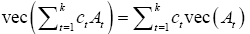
or equivalently (I) vec(cA) = cvec(A) and (II) vec(A+B) = vec(A) + vec(B). (I) is trivial since a matrix can be scaled by rows or columns. If A and B are m by n then A = [a1a2 ..an] and B = [b1b2 .. bn] so vec(A+B) = [a1T+b1T a2T+b2T.. anT+bnT]T = [a1T a2T .. anT]T + [b1T b2T .. bnT]T = vec(A) + vec(B).
A2—Derivation of the wkl statistic
The well-known result using Eq. [3] in Eq. [7] is E(b) = β. Then for every k,l, and defining  , the Chebyshev inequality is:

Therefore a 1–α confidence interval for the true βkl satisfies:

b and β have the same scale so it is clearly better to have a large estimated bkl and a small confidence interval for βkl than conversely.
Thus, we normalize the confidence interval width 2ε by bkl, and define wkl = 2ε/bkl. The coefficient of variation of the estimate bkl is ckl = σkl / bkl and  , so:
, so:

Calculating wkl for a given model requires an estimate of  , the k,l diagonal element of the covariance matrix cov(b). From Eq. [3] in Eq. [7]:

and cov(uo) is readily estimated from the residual vector eo in Eq. [6].
References
- Neuroimaging Work Group of the Alzheimer’s Association, The Use of MRI and PET for Clinical Diagnosis of Dementia and Cognitive Impairment: A Consensus Report, 2005.
- Lin JS, O’Connor E, Rossom RC, Perdue LA, Eckstrom E. Screening for cognitive impairment in older adults: A systematic review for the U.S. Preventive Services Task Force. Ann Intern Med 2013;159:601-12. [PubMed]
- Azimi-Sadjadi MR. Estimation and identification for 2-D block Kalman filtering. Signal Processing IEEE Trans 1991;39:1885-89.
- Magnus JR. eds. Linear Structures. New York: Oxford U. Press, 1988.
- Jain AK. Partial differential equations and finite-difference methods in image processing, part 1: Image representation. J Optim Theory Appl 1977;23:65-91.
- Wilks SS. eds. Mathematical Statistics. New York: Wiley, 1963:75.
- Wilks SS. eds. Mathematical Statistics. New York: Wiley, 1963:573.
- Wilks SS. eds. Mathematical Statistics. New York: Wiley, 1963:454.
- Kullback S. eds. Information Theory and Statistics. Mineola, NY: Dover Publications, 1997:6.
- Plassman BL, Langa KM, Fisher GG, Heeringa SG, Weir DR, Ofstedal MB, Burke JR, Hurd MD, Potter GG, Rodgers WL, Steffens DC, Willis RJ, Wallace RB. Prevalence of dementia in the United States: the aging, demographics, and memory study. Neuroepidemiology 2007;29:125-32. [PubMed]
- Li B, Li W, Zhao D. Multi-scale feature based medical image classification. IEEE 3rd International Conference on Computer Science and Network Technology. Chengdu, China, 2013:1182-6.
- Mahapatra D. Analyzing training information from random forests for improved image segmentation. IEEE Trans Image Process 2014;23:1504-12. [PubMed]
- Rathore S, Iftikhar MA, Hussain M, Jalil A. Classification of colon biopsy images based on novel structural features. IEEE Int Conf on Emerging Technologies. Islamabad, Pakistan, 2013:1-6.
- Box G, Jenkins G, Reinsel G. eds. Time Series Analysis, 3rd ed. Upper Saddle River NJ: Prentice Hall, 1994.
- Fuller W. eds. Introduction to Statistical Time Series. New York: Wiley & Son, 1996.
- Ljung L. eds. System Identification: Theory for the User. Upper Saddle River, NJ: Prentice Hall, 1999.
- O’Neill WD, Oroujeh AM, Merritt SL. Pupil noise is a discriminator between narcoleptics and controls. IEEE Trans Biomed Eng 1998;45:314-22. [PubMed]
- O'Neill WD, Zimmerman S. Neurologial interpretations and the information in the cognitive pupillary response. Methods Inf Med 2000;39:122-4. [PubMed]
- O'Neill WD, Trick KP. The narcoleptic cognitive pupillary response. IEEE Trans Biomed Eng 2001;48:963-8. [PubMed]
- O'Neill W, Mercer P, Sheldon S, Kotsos T. Detection of juvenile sleep deprivation by stochastic optimization of pupillographic records. Methods Inf Med 2003;42:282-6. [PubMed]
- Shuhaiber J, O’Neill W. The Diagnostic Efficacy of Left Ventricle Hemodynamic Parameters: Classifying Normal Mitral Valves Against Prosthetic Disease Proxies. Cardiovasc Eng and Tech 2012;3:112-22.
- Kullback S. eds. Information Theory and Statistics. Mineola, NY: Dover, 1997:219-22.

