
Image reconstruction of the absorption coefficients with l1-norm minimization from photoacoustic measurements
Introduction
Biomedical imaging modalities, such as optical coherence tomography (1) and optical topography (2), have garnered attentions because of their abilities to provide structural and functional information in the tissue by taking advantages of the scattering and absorption of light while it propagates through biological media. Some promising clinical applications of optical imaging are being explored. Diffuse optical tomography (DOT) (3) has been developed for the non-invasive imaging of the cerebral blood concentration (4) and for the diagnoses of breast cancers (5). By applying the near-infrared spectroscopic technique, clinically useful information, such as oxygenation state of the blood, can be obtained by DOT. Fluorescent molecular imaging also exploits the light absorption, which can be used in small animals for pre-clinical tests (6).
In recent years, photoacoustic (PA) imaging (7-9) has been developed actively. PA imaging uses the thermoelastic wave, referred to as PA pressure from the photon absorbers, such as hemoglobin and exogenous contrast agents, excited by laser irradiation (10-12). The PA imaging can be applied to aid the diagnosis of cancers by providing the functional information about the increase of the blood volume caused by angiogenesis (13). PA pressure, which has a broad frequency band, is detected by the ultrasound transducer. The photon absorbers, which generate PA pressures, are imaged by the methods such as delay-and-sum projection or circular backprojection used in conventional medical ultrasound imaging (14). The image of the photon absorbers deep inside the biological medium can be obtained with high spatial resolution, compared with conventional optical imaging. Scattering of light by the tissues strongly attenuates the light intensity and decreases the spatial resolution of optical imaging. The ultrasound is also attenuated by the tissues, but the attenuation effect is relatively small.
The amplitude of PA pressure depends on the optical absorption coefficient of photon absorbers. So, the absorption coefficient can be estimated from the PA pressure by considering light propagation. The absorption coefficient depends on molar extinction coefficient and the concentration of photon absorber. By reconstructing the distribution of absorption coefficient, the concentration of targeted absorption coefficient is estimated (15-17). The image reconstruction of the absorption coefficient is carried out by minimizing the residual error between the measured and theoretically predicted PA signals. Therefore, the numerical calculation, such as finite element method (FEM) of the PA signal, is needed for the image reconstruction. Additionally, the amplitude of the PA pressure is not strictly linear to the absorption coefficient. As a result, the non-linear optimization scheme (18) is preferable in the image reconstruction. The precise prediction of the PA signals demands computing power. However, the non-linear optimization process also involves computational cost. Considering the actual clinical use, a quick and reliable image reconstruction is desired.
The linearization of the relation between the PA signals and absorption coefficient is effective to reduce the computational cost. However, the quality of the image, such as the spatial resolution and the quantification ability, may be compromised. In this study, a linearized PA image reconstruction is attempted in numerical simulation and phantom experiment. In the meantime, the l1-norm of the reconstructed image is also minimized in the image reconstruction process in order to improve the localization of the targeted photon absorber. The latter has been used in the inverse problems and image processing in other fields (19-22). The quality of the reconstructed image with the l1-norm minimization is discussed to compare with the conventional Tikhonov regularization.
Materials and methods
Image reconstruction algorithm
To reconstruct the distribution of the absorption coefficient from the detected PA pressures, the fundamental equations dealing with the generation and the propagation of the PA pressure, which is the photon diffusion equation (PDE) and the PA wave equation, were applied. The light is scattered and absorbed by the tissues in the biological media, and the propagation of the light is the radiative transfer of the photon energy. Therefore, the radiative transfer equation (RTE) rigorously describes the light propagation (23,24). The following PDE obtained from the diffusion approximation of the RTE (25) was used in this study to reduce the calculation cost,

where D=1/(3μs’) is the diffusion coefficient with the reduced scattering coefficient μs’, μa, the absorption coefficient, Φ, the fluence rate, q0, the light source, and r, the position. The robin boundary condition is usually used with the PDE,

where n is the vector outer normal to the surface of the medium, and A is the parameter depending on the refractive index of the medium. Eq. [1] can be solved for Φ by FEM, and the PA source H, which is the absorbed photon energy, is calculated as H(r)=μa(r)Φ(r).
On the other hand, the propagation of the PA pressure in acoustically homogeneous medium is described by the PA wave equation (8,9,15),
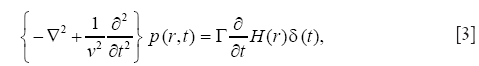
where v is the speed of the PA pressure, t, time, p, the PA pressure, and Γ, the Grüneisen parameter representing the efficiency of the PA pressure generation. Eq. [3] also can be solved by the FEM.
Let us assume that the PA pressure is detected by the PA probe which irradiates the light and detects the PA pressure at the identical position, and that the PA pressure generated directly below the PA probe is detected. The PA pressures with T time samples are detected at the K positions. According to Eq. [2], p is linear to H, the PA pressure, which is mk of the T-vector, detected at the kth position is formulated by discretizing the functions of t and r with FEM as,

where Hk is the S-vector which consists of the absorbed photon energy at S discrete positions below the PA probe, and Lk is the T×S-matrix which projects Hk to mk.
Hk is linearly approximated as, 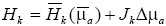 , where
  is the energy absorbed by the background medium with the absorption coefficient
  , the S×N-matrix Jk consists of the differential coefficients of Hk about , and ∆μa is the N-vector of the changes in μa at the N discrete positions in the whole medium. To reconstruct the PA source, ∆μa was reconstructed in this study. By assuming the medium is large enough to say Lj≈Lk (j≠k), and by subtracting ml form mk, we obtain (26),

then ∆μa is reconstructed by solving the following minimization problem,

where ∆m is the CT-vector consists of ∆mk,j with C of the number of the combinations of k and j. G is the CT×N matrix consists of Gk,j. f is a regularization function, and λ is the regularization parameter to adjust the effect of the regularization. When  is given, the distribution of μa is calculated as
 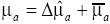 , where
  is the reconstructed ∆μa.
In this study, we compared two regularization functions: l1-norm and l2-norm of the reconstructed ∆μa. The function f employing the lp-norm is described as 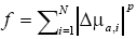 where ∆μa,i is the i th component of ∆μa (27).
Minimization of the l1-norm generally provides sparse distribution of the reconstructed solution of the inverse problems expressed by the same manner of Eq. [6]. In this study, it was expected that the photon absorber with ∆μa larger than the background was localized. In the minimization process, ∆μa,i and f were reformulated as  , respectively (26). The optimization was carried out with the non-linear conjugate gradient method.
On the other hand, minimization of the l2-norm, which is usually referred to as Tikhonov regularization (28), provides the smooth solution by reducing the influence of noise. The solution with the l2-norm minimization was obtained as,

where I is the identity matrix.
We tried the image reconstruction with following three regularizations: the l1-norm minimization with λ at the corner of the L-curve (Reg.1), the l2-norm minimization with λ at the plateau of the L-curve (Reg.2), and the l2-norm minimization with λ at the corner of the L-curve (Reg.3). Reg.2 used unusual selection of λ. The L-curve can be regarded as the plot of f as a function of the squared error e in Eq. [6]. By selecting the position where |df⁄de| is minimized, it was expected that Reg.2 would provide the smoother distribution of ∆μa than Reg.3, because Reg.2 took larger λ than Reg.3.
Conditions of the numerical simulation
Figure 1A shows the geometrical conditions for the numerical simulation. The medium of the PA pressure was a 2D square with 50 mm side. The medium had the background optical properties of μs’ =0.8 mm–1 and  . The measurement of the PA pressure was conducted at eleven positions with an equal spacing of 2 mm on the surface of the medium. There existed a photon absorber with 2 mm side and μa =0.6, 1.1 or 1.7 mm–1 on x=0 mm. The depth at which the photon absorber is located was y=5, 7 or 9 mm from the surface of the medium. The measured data ∆m used in the inversion process were calculated by the use of Eq. [5].

The 2D image reconstruction was carried out. The positions of the irradiation and the detection were identical in the image reconstruction process. The matrices of Lk and Hk were calculated with FEM with Eqs. [1] and [2]. FEM employed 10,201 nodes and 20,000 triangular elements. Gaussian noise with the standard deviation (SD) of 10% of the maximum of ∆m was added. The image reconstruction was carried out on pixel basis as described in the literature (29). A single pixel consisted of 25 nodes. Three trials of the image reconstruction with Regs.1, 2 or 3 were carried out for each combination of μa and the depth of the photon absorber.
Conditions of the phantom experiment
Figure 1B shows the schema of the phantom experiments. The background of the phantom was an aqueous solution of the intralipid and indocyanine green (ICG). The optical properties of the phantom was adjusted to μs’ =0.8 mm–1 and (30). The tube with an inner diameter of 1 mm and an outer diameter of 2 mm placed in the phantom as a photon absorber. The tube contained the intralipid and ICG with μs’ =0.8 mm–1 and μa =0.6, 1.1 or 1.7 mm–1. The depth of the photon absorber was y=5, 7 or 9 mm.
A tunable Ti:sapphire laser pumped by the second harmonic of a Q-switch Nd:YAG laser (LT-221 and LS-2134, Lotis Tii, Minsk, Belarus) was used for the laser irradiation. The laser light was introduced into the optical fiber. The optical fiber was installed in the cylindrical PA probe which had a ring shaped piezoelectric film P(VDF-TrFE) (KF piezo-film, Kureha Corp., Tokyo, Japan) on the edge of the PA probe (Figure 2). The edge of the optical fiber was placed at the center of the piezoelectric film so that the laser irradiation and the PA detection were conducted at the identical position. The energy of the light from the optical fiber was 4 mJ/pulse. The PA pressure was detected at the eleven positions aligned perpendicularly to the long axis of the tube of the photon absorber with an equal spacing of 2 mm. The measured data were acquired by the digital oscilloscope (DSO8104A, Agilent Technologies, Santa Clara, CA) via the amplifier (SA-220F5, NF Corp., Yokohama, Japan). The image reconstruction was carried out in 2D with the same manner of the numerical simulation.

Results
Numerical simulation
Figure 3 shows the reconstructed images using the regularization methods in the case of μa =1.1 mm–1 and the depth of 7 mm of the photon absorber. Reg.1 reconstructed the localized μa distribution. The reconstructed value and the positions of the photon absorber were corrected in all cases with a combination of μa and depths. Reg.2 also reconstructed the photon absorber at the correct position, although the reconstructed value of μa was smaller and the distribution was slightly broader than the true one. The influence of the noise was not seen in the images reconstructed with Regs.1 and 2.

Reg.3 reconstructed the maximum value of μa at the correct position of the photon absorber. Although Reg.3 used Tikhonov regularization, the influence of the noise was seen at the deep positions in the medium. The reconstructed images in all cases with various μa and the depths of the photon absorber had similar characters depending on the regularization methods.
Figure 4 shows the signal-to-noise ratio (SNR) of the reconstructed μa of the photon absorber. SNR1 was defined as SNR1 =10 log10 (∆μa,max /σ1)2, where ∆μa,max is the average of the maximum reconstructed ∆μa and σ1 is SD of ∆μa,max estimated from the three trials with each of Regs1, 2 and 3. Figure 4A shows the averages of SNR1 among the cases with the depths of 5, 7, 9 mm which were calculated for each of the cases with μa =0.6, 1.1 or 1.7 mm–1. The averages of SNR1 among the cases with μa =0.6, 1.1 or 1.7 mm–1 calculated for the cases with the depths of 5, 7 or 9 mm are shown in Figure 4B. SNR1 were in the range from 30 to 40 dB in all cases. This means that ∆μa,max was approximately 60 times larger than the error due to the measurement noise. The dependences of SNR1 on the depth, ∆μa,max of the photon absorber or the regularization methods were not seen in Figure 4.

On the other hand, Figure 5 shows SNR2 defined as SNR2 =10 log10 (∆μa,max/σ2)2, where σ2 was the total of the reconstructed |∆μa| except ∆μa,max. In the same manner as SNR1, the averages of SNR2 calculated for the cases with μa =0.6, 1.1 or 1.7 mm–1 are shown in Figure 5A, and those calculated for the depth of 5, 7 or 9 mm are in Figure 5B. Reg.1 obtained SNR2 of about 25 dB in all cases, while SNR2 of Regs.2 and 3 were about –10 and –15 dB, respectively. ∆μa of the photon absorber reconstructed with Reg.1 was 20 times larger than the artifacts in the reconstructed image caused by the noisy measurement data, while the artifacts were larger than the reconstructed ∆μa of the photon absorber in the images reconstructed with Regs.2 and 3.

Phantom experiment
Figure 6 shows the reconstructed images in the case with μa =1.1 mm–1 and the depth of 7 mm of the photon absorber of the phantom experiments. The reconstructed values were calibrated by the regression line fitting the give sets of the true μa of the photon absorber and the averages of the reconstructed values at the depths of 5, 7 and 9 mm. The maximum value of μa was reconstructed at the correct position for all combinations of μa and the depths of the photon absorber by each of the regularization methods. The reconstructed images demonstrated that Reg.1 reduced the influence of noise and localized μa distribution more strongly than Regs.2 and 3 as well as in the previous numerical simulation. The quality of the reconstructed image was improved by the l1-norm minimization, although the reconstructed photon absorber had the area larger than true one. SNR2 of the images reconstructed with Regs.1, 2 and 3 were –12.4, –23.0 and –31.3 dB, respectively. The phantom experiment showed that Regs. 1 can obtain larger SNR2 than Regs.2 and 3.

μa of the photon absorber reconstructed with Reg.1 is plotted as a function of the true μa of the photon absorber for the numerical simulation and the phantom experiment in Figure 7A,B, respectively. In both of the numerical simulation and phantom experiment, the reconstructed μa of the photon absorber reflected the increase of the true μa with linearity on some level. Regs.2 and 3 also showed the similar results. However, μa,max depended on the depth of the photon absorber in the phantom experiment. The deeper position the photon absorber was placed at, the smaller the reconstructed μa of the photon absorber was, while μa,max did not depend on the depth of the photon absorber in the numerical simulation.

Discussion
Artifacts appeared in the images reconstructed with Reg.3 in both the numerical simulation and the phantom experiment. The image reconstruction of μa from the PA pressure took the light propagation in the medium into account. At the deeper position, Φ became small owing to scattering and absorption of the light. To reconstruct μa of the photon absorber in various depths correctly, the image reconstruction algorithm compensated the rapid decrement of Φ. This function of the image reconstruction algorithm amplified the measurement noise observed at the late times. The time at which the PA pressure was detected corresponds to the distance from the detector to the photon absorber. So, the influence of the measurement noise observed at the late times appeared as artifacts at the deeper positions. The artifacts were reduced by Reg.2, because λ was larger, and the smoothing effect of the Tikhonov regularization of Reg.2 was stronger than that of Reg.3.
The photon absorber was reconstructed with large SNR1 at the correct position by Regs.1, 2 and 3, regardless of μa and the depths of the photon absorber, although SNR1 fluctuated owing to the measurement noise. SNR2 quantitatively shows that Reg.1 strongly suppressed the influence of measurement noise on the reconstructed image, regardless of μa and the depths of the photon absorber. Reg.1 was superior to Regs.2 and 3 in the sense of SNR2. Reg.2 is better to be used to reduce the influence of measurement noise than Reg.3 which used the conventional parameter selection for the Tikhonov regularization. SNR2 in the phantom experiment was smaller than that in the numerical simulation, because the reconstructed large μa distributed larger than true one and some artifact appeared owing to noise.
Through the numerical simulation and the phantom experiment, Reg.1 obtained the reconstructed image effectively suppressing the influence of the measurement noise, because the reconstructed distribution of ∆μa needed to be sparse to minimize the l1-norm. It is known that the regularization minimizing the lp-norm with p smaller than unity generally obtains sparse solutions of inverse problems (19,20). It was demonstrated that the l1-norm minimization provided the sparse solution robust to noise by the evaluations of the reconstructed images with SNR1 and SNR2. The characteristic of the l1-norm minimization in obtaining the sparse solution can be useful to image small imaging targets, such as micro-blood vessels and the cancers at early stage labeled by the contrast dye in a small region. The robustness to noise of the image reconstruction with the l1-norm minimization can be helpful for the image reconstruction of small imaging targets, because the PA pressure from the small imaging target is small and the SNR of the PA pressure is low.
Some side effects of the powerful regularization should be noticed. Regs.1 and 2 may suppress the smaller PA signals from the photon absorber embedded deeply inside the medium. Additionally, the strong localization effect of Reg.1 can reconstruct the distribution of the photon absorber smaller than true ones when the true photon absorbers are broadly distributed. The PA image reconstructed with a certain regularization method should be carefully interpreted for the medical diagnosis by considering the characteristics of the regularization method.
Figure 6A shows that Reg.1 quantitatively reconstructed μa of the photon absorber when the image reconstruction algorithm fit the physical model of the PA measurement. The difference between Figure 6A,B can occur because of the 2D image reconstruction used in this study. In the phantom experiment, the light and the PA pressure propagated in larger volume of 3D medium than that of 2D medium. Then, the excitation light and PA pressure from deeper position in 3D medium was attenuated more strongly than that predicted in 2D medium.
However, μa at the depth of 5 mm was twice as large as that of 9 mm, while the PA pressure from the depth of 5 mm was about 5-fold of that of 9 mm in the phantom experiment. This means that the 2D image reconstruction compensated the attenuation of the light and PA pressure to some extent, although the 2D image reconstruction cannot recover them perfectly.
Conclusions
In this study, the effect of the l1-norm minimization on the image reconstruction from the PA measurement was compared to the Tikhonov regularization. By the numerical simulation and the phantom experiment, we demonstrated that the l1-norm minimization localized the distribution of the absorption coefficient and clearly imaged the photon absorber in the medium. The influence of noise on the reconstructed image was sensible by using the Tikhonov regularization in this study. The image reconstruction with the regularization minimizing the l1-norm is useful for the PA measurement when the distribution of the photon absorber is sparse and the signal-to-noise ratio of the detected PA pressure is low. The l1-norm minimization can be used for the nonlinear image reconstruction algorithm.
Acknowledgements
This work was partially supported by JST collaborative Research Based on Industrial Demand (In vivo Molecular Imaging: Towards Biophotonics Innovations in Medicine) and JSPS KAKENHI (Grant Number 24760314). The authors thank Hiroaki Ishihara for his assistance in the phantom experiment.
Authors’ contribution: S.O. designed overall study and wrote the paper. S.O. constructed the image reconstruction algorithm and carried out the numerical simulations. S.O., T.H. and T.K. constructed the experimental setup, collected and analyzed the data. S.O., T.H., T.K. and M.I. discussed and edited the paper. M.I. supervised this study.
Disclosure: The authors declare no conflict of interest.
References
- Yin X, Chao JR, Wang RK. User-guided segmentation for volumetric retinal optical coherence tomography images. J Biomed Opt 2014;19:086020. [PubMed]
- Wang S, Shibahara N, Kuramashi D, Okawa S, Kakuta N, Okada E, Maki A, Yamada Y. Effect of Spatial Variation of Skull and Cerebrospinal Fluid Layer on Optical Mapping of Brain Activities. Opt Rev 2010;17:410-20.
- Gibson AP, Hebden JC, Arridge SR. Recent advances in diffuse optical imaging. Phys Med Biol 2005;50:R1-43. [PubMed]
- Fukuzawa R, Okawa S, Matsuhashi S, et al. Reduction of image artifacts induced by change in the optode coupling in time-resolved diffuse optical tomography. J Biomed Opt 2011;16:116022. [PubMed]
- Yates T, Hebden JC, Gibson A, Everdell N, Arridge SR, Douek M. Optical tomography of the breast using a multi-channel time-resolved imager. Phys Med Biol 2005;50:2503-17. [PubMed]
- Okawa S, Yano A, Uchida K, Mitsui Y, Yoshida M, Takekoshi M, Marjono A, Gao F, Hoshi Y, Kida I, Masamoto K, Yamada Y. Phantom and mouse experiments of time-domain fluorescence tomography using total light approach. Biomed Opt Express 2013;4:635-51. [PubMed]
- Wang LV, Hu S. Photoacoustic tomography: in vivo imaging from organelles to organs. Science 2012;335:1458-62. [PubMed]
- Li C, Wang LV. Photoacoustic tomography and sensing in biomedicine. Phys Med Biol 2009;54:R59-97. [PubMed]
- Xu M, Wang LV. Photoacoustic imaging in biomedicine. Rev Sci Instrum 2006;77:041101.
- Hu S, Wang LV. Photoacoustic imaging and characterization of the microvasculature. J Biomed Opt 2010;15:011101. [PubMed]
- Erpelding TN, Kim C, Pramanik M, Jankovic L, Maslov K, Guo Z, Margenthaler JA, Pashley MD, Wang LV. Sentinel lymph nodes in the rat: noninvasive photoacoustic and US imaging with a clinical US system. Radiology 2010;256:102-10. [PubMed]
- Wang X, Pang Y, Ku G, Xie X, Stoica G, Wang LV. Noninvasive laser-induced photoacoustic tomography for structural and functional in vivo imaging of the brain. Nat Biotechnol 2003;21:803-6. [PubMed]
- Heijblom M, Piras D, Xia W, van Hespen JC, Klaase JM, van den Engh FM, van Leeuwen TG, Steenbergen W, Manohar S. Visualizing breast cancer using the Twente photoacoustic mammoscope: what do we learn from twelve new patient measurements? Opt Express 2012;20:11582-97. [PubMed]
- Sperl JI, Zell K, Menzenbach P, Haisch C, Ketzer S, Marquart M, Koenig H, Vogel MW. Photoacoustic image reconstruction: a quantitative analysis. Proc SPIE 2007;6631:663103.
- Cox B, Laufer JG, Arridge SR, Beard PC. Quantitative spectroscopic photoacoustic imaging: a review. J Biomed Opt 2012;17:061202. [PubMed]
- Laufer J, Cox B, Zhang E, Beard P. Quantitative determination of chromophore concentrations from 2D photoacoustic images using a nonlinear model-based inversion scheme. Appl Opt 2010;49:1219-33. [PubMed]
- Yuan Z, Wang Q, Jiang H. Reconstruction of optical absorption coefficient maps of heterogeneous media by photoacoustic tomography coupled with diffusion equation based regularized Newton method. Opt Express 2007;15:18076-81. [PubMed]
- Saratoon T, Tarvainen T, Cox BT, Arridge SR. A gradient-based method for quantitative photoacoustic tomography using the radiative transfer equation. Inverse Problems 2013;29:075006.
- Okawa S, Hoshi Y, Yamada Y. Improvement of image quality of time-domain diffuse optical tomography with l sparsity regularization. Biomed Opt Express 2011;2:3334-48. [PubMed]
- Okawa S, Ikehara T, Oda I, Yamada Y. Reconstruction of localized fluorescent target from multi-view continuous-wave surface images of small animal with lp sparsity regularization. Biomed Opt Express 2014;5:1839-60. [PubMed]
- Xu P, Tian Y, Chen H, Yao D. Lp norm iterative sparse solution for EEG source Localization. IEEE Trans Biomed Eng 2007;54:400-9. [PubMed]
- Chang CH, Ji JX. Improving multi-channel compressed sensing MRI with reweighted l 1 minimization. Quant Imaging Med Surg 2014;4:19-23. [PubMed]
- Tarvainen T, Kolehmainen V, Arridge SR, Kaipio JP. Image reconstruction in diffuse optical tomography using the coupled radiative transport-diffusion model. J Quant Spectrosc Radiat Transfer 2011;112:2600-8.
- Fujii H, Okawa S, Yamada Y, Hoshi Y. Hybrid model of light propagation in random media based on the time-dependent radiative transfer and diffusion equations. J Quant Spectrosc Radiat Transfer 2014;147:145-54.
- Arridge SR. Optical tomography in medical imaging. Inverse Problems 1999;15:R41-93.
- Okawa S, Hirasawa T, Kushibiki T, Ishihara M. Reconstruction of the optical properties of inhomogeneous medium from photoacoustic signal with lp sparsity regularization. Proc SPIE 2013;8581:858135.
- He Z, Cichocki A, Zdunek R, Xie S. Improved FOCCUS Method With Conjugate Gradient Iterations. IEEE Trans Signal Process 2009;57:399-404.
- Vogel CR. Computational Methods for Inverse Problems (Frontiers in Applied Mathematics), Philadelphia, 2002.
- Okawa S, Hirasawa T, Kushibiki T, Ishihara M. Numerical Evaluation of Linearized Image Reconstruction Based on Finite Element Method for Biomedical Photoacoustic Imaging. Opt Rev 2013;20:442-51.
- van Staveren HJ, Moes CJ, van Marie J, Prahl SA, van Gemert MJ. Light scattering in Intralipid-10% in the wavelength range of 400-1100 nm. Appl Opt 1991;30:4507-14. [PubMed]

