Fully automatic deep learning trained on limited data for carotid artery segmentation from large image volumes
Introduction
Stroke is a pervasive and critical cause of morbidity and mortality that affects the global population (1). Atherosclerotic disease in the carotid artery bifurcation area is the primary cause of stroke in 25% of patients with this condition (2). Carotid bifurcation is where the common carotid artery (CCA) divides into the external carotid artery (ECA) and internal carotid artery (ICA). Due to the blood vortex that forms in this bifurcation area and the increased shear force on the vessel wall, atherosclerotic plaque, which is composed of fat, cholesterol, calcium, and other substances found in the blood, accumulates, resulting in a narrowing or blockage of blood flow to the brain.
The degree of stenosis in the carotid artery is a significant factor that influences clinical decisions regarding surgical treatments, such as stenting or endarterectomies. Digital subtraction angiography (DSA) is regarded as the gold standard for diagnosing carotid stenosis severity, and which is a slight risk factor contributes to neurological deficits such as ischemic stroke. Computed tomography angiography (CTA) is the most accurate noninvasive imaging technique for evaluating carotid stenosis, with color Doppler ultrasonography and magnetic resonance angiography (MRA) being less accurate (3). However, the first step towards quantitatively assessing stenoses post-imaging is to perform segmentation of the carotid bifurcation and exclude the plaques. This task is difficult, even for experienced radiologists, and there is high interobserver and intraobserver variability in segmentations (4,5). Automatic and accurate methods of carotid bifurcation segmentation are therefore urgently needed to better quantify carotid stenoses.
The first step of traditional carotid vessel segmentation methods is to extract centerlines through the vessels. According to a review of vascular lumen segmentation in MRA and CTA images (6), graph cuts, level sets, and active shape models are three basic methods frequently used to extract vessels. Most traditional segmentation techniques are semiautomatic, such as those used by Tang et al. and Hemmati et al. (7-9). These are semiautomatic because in the initialization stage they use three seed points located in the CCA, ICA, and ECA that are previously selected by human experts. Cuisenaire et al. (10) developed a novel initial centerline extraction technique to eliminate reliance on manual seed points. A patient-adapted anatomical model was used to initialize and constrain the algorithm to produce centerlines (10); however, the model failed in cases where vessels were fully occluded, reflecting severe stenoses that required additional attention. This model therefore lacked the robustness required for carotid segmentation. Bozkurt et al. (11) proposed region-growing and random walk algorithms that segment the bone region first and then the vessel once the bone is removed, as bone can be easily confused with the target object. Similarly, Wu et al. (12) addressed the confusion between bone tissue and blood vessels by removing bone structures prior to studying the segmentation of head and neck vessels in CTA images. This approach is fully automatic, because seeds are selected from experimentally determined intervals according to the local histogram, and good agreement with expert manual measurements was achieved. Additionally, Tavares et al. (13-19) proposed a series of novel methods related to automatic artery segmentation, the classification of calcified regions, and hemodynamics in multi-modality medical images.
In recent years, the deep neural network (DNN) has shown the ability to learn a hierarchical representation of raw input data and has demonstrated excellent performance in image segmentation tasks (20-23). U-Net (24) is the most frequently used network applied in semantic segmentation of medical images and employs skip connections to combine high-resolution features and upsampled outputs, which yields good performance for two-dimensional (2D) images. However, it is difficult to build deeper networks that have high discriminative power for volumetric data due to the huge computational expense. Some researchers have attempted to extend 2D convolutional neural networks (CNNs) to volumetric applications using adjacent slices (25), orthogonal planes (26,27), and multiview planes (28) to capture the 3D contextual information of images. However, the 3D features that represent images in these models have not been explored in depth. Some studies have used 3D CNNs and fed volumetric data directly into the networks to develop variants of the 3D version of U-Net (29-31). However, DNNs have rarely been adopted for carotid vessel lumen segmentation, especially in 3D CTA images. Zheng et al. (32) combined Harr wavelet features with deep learning image features to detect carotid bifurcation points in 3D head and neck CT images. Other studies (33-35) have focused on 2D carotid ultrasound images, using CNNs to segment the intima and adventitia of the arterial wall in order to assess the intima-media thickness (IMT). Possible reasons for the absence of deep learning for volumetric segmentation of carotid lumens include the unavailability of annotated data and the trade-off between the network receptive field and limited computing memory for 3D images. Furthermore, arteries are easily confused with nearby structures, such as veins and bone tissue, which increases segmentation difficulty.
In this study, we applied fully automatic semantic segmentation of the carotid bifurcation lumen in CTA images. Firstly, we used residual connections, dilated convolutions, and a deep supervision strategy, integrating these methods into a 3D variant of U-Net, called CarotidNet. Secondly, we provided a two-phase strategy to segment tiny target objects from large image volumes. This two-phase strategy included an object localization stage and a precise segmentation stage. These two stages used the same network, and the second training stage was fine-tuned using the pretrained model from the first stage. Thirdly, we combined Dice loss and focal loss to address the extreme distribution imbalance between—as they are labelled in the annotations—background voxels and carotid lumen voxels.
The remainder of the paper is organized as follows. Section II describes the study materials and methods, including an introduction to the dataset, data preprocessing steps, two-phase strategy, proposed network architecture, and combined loss functions. We present and analyze the results in section III and discuss the study limitations and directions of future work in section IV. Finally, conclusions are drawn in section V.
Methods
In this section, we introduce our deep learning model for the segmentation of carotid bifurcations in head and neck CTA images. Our method relies on a two-stage cascade network where both stages have the same structure. The first network aims to extract the region of interest (ROI), namely, the bounding box of carotid bifurcation vessels, from the entire CTA volume. The second network focuses on the precise segmentation of the obtained ROI.
Dataset
The Medical Image Computing and Computer Assisted Intervention (MICCAI) 2009 Workshop on Carotid Lumen Segmentation and the Stenosis Grading Challenge (2) provide a publicly available source of 56 head and neck CTA images, of which 15 are training images and 41 are testing images with actual annotations that are not publicly available. These images show varying degrees of stenosis and were acquired from three medical centers. Due to diverse scanners, image resolutions, and size characteristics, the in-plane pixel size ranges from 0.23 to 0.547 mm, the slice thickness is either 1 or 0.9 mm, the z-spacing ranges from 0.45 to 0.6 mm, and the number of slices ranges from 395 to 827.
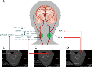
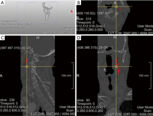
There are two carotid bifurcations in each image, but each volume annotation from the dataset is only applicable to one side (Figure 1A,B). The annotated region covers 20 mm below the CCA bifurcation slice, 40 mm above the ICA bifurcation slice, and between 10 and 20 mm above the ECA bifurcation slice (Figure 1C,D). Figure 2 shows a case of original CTA images with annotations from the training set.
Preprocessing
It is not possible to use an entire fine-resolution image for segmentation due to the large data volume; there is a trade-off between computational memory and resolution loss during resampling. We therefore used a two-stage resampling strategy where both stages are resampled from the original images. In the first stage, we resampled them to a size of 256×256×160 and a spacing of 1.2 mm × 1.2 mm × 2.4 mm. In the second stage, the resampling size was 512×512×640, and the spacing was 0.6 mm in each dimension. The emphasis of the first stage was to localize the carotid artery; therefore, resolution loss was acceptable in this step. The second stage focused on precise segmentation of the region identified in the first stage from the original images, so the processing resolution was relatively high. In the resampled image with a size of 256×256×160 in the first stage, the center size of 128×128 in the x-y in-plane region was enough to cover the scope of the carotid bifurcation. Moreover, because the ground-truth annotation was applicable for either side, we further reduced the first stage volume to the left or right 5/8 of the center region, giving a size of 80×128×160. The reason we did not reduce the images to half the original size was to include some cases with minor shifts.
In the intensity normalization step, we first applied Otsu thresholding to each image to obtain a mask excluding spaces filled with air. Each volume was subsequently subtracted from the mean and divided by the standard deviation in the context of the mask. Finally, the image intensity was clipped to the range [−5, 5] and then rescaled to [0, 1].
Network architecture
Standard U-Net architecture is composed of the contraction path and the expansion path. In the contraction path, the feature channels double progressively as the size is halved four times by max pooling. In the expansion path, the feature channels halve progressively as the size is doubled until the original size is restored. The skip connections of the corresponding levels of features combine the location details of the former image and the semantic discriminative information of the latter image to perform semantic segmentation with high location accuracy. The skip connections also allow errors to easily propagate into the contraction path layers and facilitate the training process.
A deep network architecture with many parameters theoretically has greater discriminative power than a basic architecture (36), but may experience the vanishing gradient problem during the training process (37). To address this, He et al. (37) proposed a network stacked with residual units where the identity mappings (38) share similar skip connections to enable rapid error propagation. A deep supervision strategy that uses auxiliary supervision in intermediate layers (39,40) was also suggested to simplify training and potentially improve performance. When the network extends from 2D to 3D, the model can leverage the interslice context of CTA images and make better predictions for a volumetric patch of a scan (41). However, maintaining a proper field-of-view and deeper network in 3D would result in rapid growth in demand for computational resources, especially GPU memory. The cost of training would therefore greatly increase (42). However, we employed residual connections along with a deep supervision strategy in our network structure to facilitate the preservation of the gradient norm, which resulted in stable back-propagation (43).
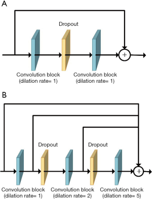
Dilated convolution can expand the receptive field without losing resolution or coverage in dense prediction (44). Influenced by the notion of hybrid dilated convolution proposed by Wang et al. (45), which extracts multiscale features and avoids the gridding effect (46), we replaced the convolutions at the transitions between the contraction and expansion paths with cascaded dilated convolutions to capture a larger context, especially in 3D backgrounds (Figure 3).
Residual connections, deep supervision, and dilated convolutions are three recent advances in deep learning, and CarotidNet leverages their corresponding strengths based on U-Net. The convolution layers all have strides of 1×1×1, dilation rates of 1×1×1, and padding to maintain their original sizes. Given the relevant memory and volume limitations, our batch size was either 1 or 2, so we replaced batch normalization with instance normalization. Each convolutional block contained a 3D convolution layer with a kernel size of 3×3×3, followed by an instance normalization layer and subsequent leaky-ReLU nonlinearity. We adopted pre-activation residual connections between convolution blocks in the contraction path to avoid performance degradation in the DNN. These pre-activation residual connections are called residual convolution modules (the blue arrow in Figure 4). We used a spatial dropout layer between convolution blocks to mitigate overfitting, and we used convolution blocks with a stride of 2×2×2 (the red arrow in Figure 4) to connect the residual convolution module for downsampling and to double the number of feature maps. To further enlarge the network receptive field, cascaded dilated convolutions with dilation rates of 1, 2, and 5 were used in the deepest layer of the contraction path. These were called the dilated convolution modules (the yellow arrow in Figure 4).
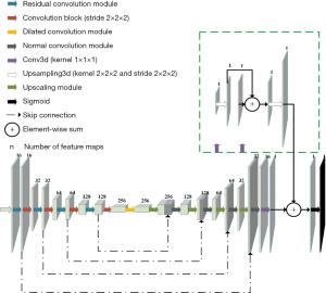
In the expansion path, the upscaled module (the white arrow in Figure 4) contained an upsampled 3D layer (kernel =2×2×2; stride =2×2×2) and a convolution block that halved the feature channels. We then concatenated the features with those of the corresponding levels in the contraction path and applied a normal convolution module (the black arrow in Figure 4) consisting of two cascade convolution blocks. To mitigate gradient explosions and vanishing issues, and to facilitate faster convergence, we employed a deep supervision strategy (47) in the expansion path by integrating the outputs at different levels of this path that were produced by a convolutional layer (kernel =1×1×1) and a subsequent upsampling layer (kernel =2×2×2; stride =2×2×2). As shown in Figure 4, we combined the deep blocks with shallow blocks using sequential summation. Finally, we applied sigmoid nonlinearity to perform probabilistic segmentation with values ranging from 0 to 1.
Training and testing scheme
As the volumetric data set is too large to feed into the network, even if there is only one whole volume in a batch, some studies (48-50) have used patch-based methods to address this issue. These methods extract small regions called patches from an image to be used as inputs for both training and testing. However, in our study, the carotid bifurcation lumen accounted for a small percentage of the whole image. With respect to these patch-based methods, a large quantity of patches will only have negative labels if they are randomly selected. Additionally, datasets tend to be further imbalanced due to patch overlaps. We therefore divided the task into two phases: the localization phase and the segmentation phase.
As the proportion of positive labels in training data during the segmentation phase was higher than that during the localization phase, we first trained the segmentation phase network. The training data volumes were regions 144×144×144 in size at the center of the annotation bounding box that was extracted during the second stage, as noted above in the preprocessing section, resulting in a trained segmentation model. We then trained the network for the localization phase by feeding in 80×128×160 size volumes from the first stage and adjusting the weights initialized from training results in the segmentation phase, which produced a trained localization model.
During the testing phase, we first passed the 80×128×160 size volume with 1.2 mm × 1.2 mm × 2.4 mm spacing to the localization model and extracted the carotid location. Based on the carotid location, we further extracted 144×144×144 size volumes according to the center of the carotid bounding box and fed the extracted volumes into the segmentation model.
Loss function
Like most biomedical segmentation datasets, our dataset suffered from a dominant distribution of negative labels, which may have caused the segmentation network to be biased towards the background. To better understand the imbalance between positive and negative labels, for every volume in the training set, we calculated the proportion of voxels that were labeled as positive and negative by experts. Table 1 displays these statistics. Note that the samples calculated in resampled space A were 80×128×160 size volumes extracted from the first stage, and the samples calculated in resampled space B were 144×144×144 size volumes extracted from the second stage.

Full table
Table 1 shows how the training set used during the localization phase was more imbalanced than that used in the segmentation phase. This explains why we trained the segmentation phase network first. To alleviate the negative impact of class imbalance during the training process, we combined Dice loss (29) and focal loss (51), because Dice loss attaches more importance to overlapping parts of the predicted and annotated volumes while focal loss focuses on misclassified examples. The Dice loss derived from the Dice similarity coefficient (DSC) is defined as follows:
[1]
where
The focal loss, which decreases the contribution of well-classified examples to the objective function, is defined as follows:
[2]
where γ, pt, and αt meet the following conditions.
[3]
[4]
[5]
We set α and γ as 0.25 and 2, respectively, as recommended in experiments by Lin et al. (51). The total loss, L, in our method was the summation of Dice loss and adjusted focal loss as follows:
[6]
where
Implementation details
This method was implemented in Python using Keras (52) with a TensorFlow (53) backend. There were 8,269,579 parameters in the overall network. We adopted the Adam optimizer with an initial learning rate of 1e–4 during the segmentation phase and 5e–5 during the localization phase.
Because there were only 15 volumes in the training set, it was essential to augment the original training dataset to improve robustness and prediction accuracy. To reduce excessive storage requirements, we augmented data on the fly. We performed a random combination of augmentation operations on images before generating training batches to feed into the network, including translation in the range of [−15, 15] voxels, rotation with angles in the range of [−15, 15] degrees, flipping along the x-axis, and resizing in the range of [0.8, 1, 2].
We randomly selected three volumes from the training set each from three distinct medical centers as a validation set and adopted an early stopping strategy with a patience of 50 for training purposes. For postprocessing, we first binarized the final probabilistic heat map with a threshold selected according to the validation set. We then optimized the results by performing connected component analyses on the binarized images to remove some isolated false-positive regions and to obtain the target object segmentation results. Finally, we resampled the segmented images to each original space to compare them with the gold standard of the MICCAI challenge 2009.
Results
Evaluation metrics
We used the DSC as the main metric to evaluate the performance of our carotid bifurcation segmentation method. DSC is defined as follows:
[7]
where
DSC focuses on the overlap of two volumes to assess the corresponding geometric surface distance. The mean surface distance (MSD) and Hausdorff surface distance (HSD) (2) are also included in the evaluation metrics. All three metrics were computed by the MICCAI challenge 2009 website’s internal algorithm from the binary segmentation results we submitted.
Ratios of focal loss in the total loss function
Although the MICCAI 2009 Challenge was finished at the time the current study was being conducted, registered users could still submit segmentation results to the MICCAI website (54) and contact the organizers to audit these uploaded results. The organizers then made the evaluation metrics available to the registered user. However, to obtain testing results every time they were required, permission was needed from the organizers to view the evaluation metrics on the website, which would make it an off-line process. We therefore reproduced the segmentation output of the test set used by Tang et al. in a previous work (7) of published results of the challenge, and used this data to establish the auxiliary labels as an auxiliary standard. We then calculated the evaluation metrics to determine the proper ratio of focal loss in the total loss function.
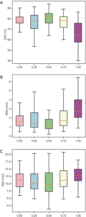
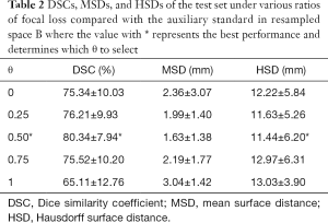
For the test set, the average DSC of the auxiliary labels compared with the gold standard was 90.2%, which indicates the auxiliary labels achieved good agreement with the gold standard. Figure 5 and Table 2 show the average DSCs of the network prediction results for different θ selections compared with the auxiliary labels (i.e., the auxiliary standard).
Full table
In cases where the ratio of Dice loss and focal loss in the loss function was 2:1, or θ=0.5, the segmentation performance for the test set was best when the average DSC, compared with the auxiliary standard, was 80.34%. Therefore, 0.5 was chosen as the best ratio of focal loss to Dice loss in the total objective function. In the following section, hybrid loss is referred to as the combined objective function of Dice loss and focal loss with θ set as 0.5.
Comparison with the original 3D U-Net and weighted cross-entropy loss
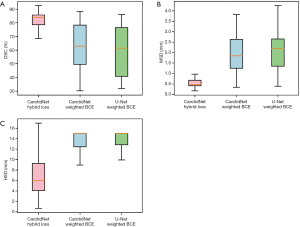
We also trained the CarotidNet with weighted binary cross-entropy loss and extended the original U-Net to 3D with weighted binary cross-entropy. We then compared these results with that of CarotidNet trained with hybrid loss. In the weighted binary cross-entropy function, we set the positive weight as the ratio between negative voxels and positive voxels calculated with the training set. To illustrate the effect of the designed network structure and loss function, we compared the segmentation performance of the three models discussed above. The DSC, MSD, and HSD were three measures used to evaluate the performance of the segmentation methods; the results are shown in Table 3 and Figure 6.

Full table
Visualization of the test set
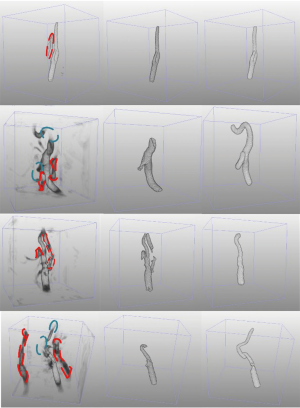
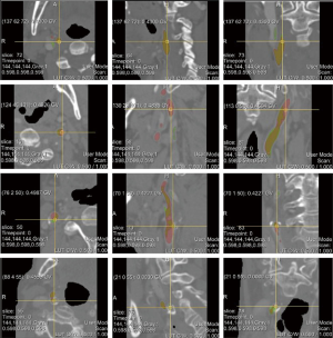
Figure 7 visualizes the 3D reconstructed images of four segmentation results generated by CarotidNet with hybrid loss for four different cases from the test set. The first row in the figure depicts the case with the best performance for the proposed method; the other three cases showed worse performance. The best case had the highest performance across all three measures among the test sets. One or two measures of the proposed method in the other three cases ranked last of all the measures among test methods. The columns from left to right show the direct prediction probability maps of the network: the red dotted lines indicate false-positive areas, and the green ellipses denote false-negative voxels, the segmentation results after postprocessing, and segmentations of the auxiliary labels. Note that the false-positive and false-negative voxels here were determined based on the auxiliary labels, as the actual annotations were not available to the public. Mismatches may therefore occur, particularly in the third row where the auxiliary labels achieved a 71.4% DSC compared with the gold standard, which was the worst performance observed. The poor performance evident in the second and fourth rows were primarily due to false-negative voxels, particularly those in lumens with high curvature. Figure 8 shows the corresponding 2D slices.
Leave-one-out cross-validation
As there were only 15 cases in our training dataset and 41 cases in the testing dataset, it was unclear to what degree the segmentation performance was restricted by the training dataset’s limited size. To reduce the impact of the small training dataset size on model performance, we used the segmentations reproduced from the auxiliary labels (7) based on the test set together with the training set to perform leave-one-out cross-validation. Using this approach, the training dataset was enlarged to 55 and the testing dataset was reduced to 1 with every validation. The results are presented in Table 4. The average DSC increased from 82.26% to 86.45%, and the average MSD and HSD decreased significantly.

Full table
Impacts of preprocessing and postprocessing
Due to the variety of scanning parameters for CTA images, we needed to resample the images to achieve uniform spacing for the training process. When we submitted the test set results to the MICCAI website, however, the segmented outputs had to have the same spacing as the corresponding original images. In other words, we resampled twice in the overall process. To evaluate the error associated with resampling, we resampled the resampled ground-truth annotations with a spacing of 0.6 mm × 0.6 mm × 0.6 mm to the original spacing and evaluated the results based on three measures compared with the gold standard. This process was only performed for the training set, because the gold standard of the test set was unknown. The evaluation metrics are shown in Table 5. Note that Observers A, B, and C are human experts. The gold standard was generated using the average of their annotations.

Full table
For the training set, resampling the results twice creates an approximately 6.9% error in the DSC, which theoretically suggests that the maximum DSC of the proposed method can only reach approximately 93.1%. The third row of Figure 7 indicates that there are possible side branches in our predictions. However, our method primarily focuses on the application of deep learning, not removing side branches in postprocessing. Our postprocessing stage primarily involved binarization, and the connected component analysis mainly used intensity information from the probability maps. In traditional image processing methods (55,56), centerlines and shape information are usually used to remove outliers. Given these two approaches, an 82.3% DSC demonstrated that the performance of the proposed method was highly consistent with the gold standard.
The binarization scheme is rigid in postprocessing because the threshold is the same for each voxel in each volume. To address this, Wang et al. (57) proposed a threshold map and direct introduction of the error associated with the threshold in the objective function so that the network can learn a probability heat map and a corresponding threshold map simultaneously. In other words, the thresholds were different for each voxel in each image, and therefore the binarization scheme was flexible and locally related.
Comparison with other fully automatic methods
To the best of our knowledge, only three fully automatic carotid segmentation methods currently exist, including ours. Although the first fully automatic method (10) reached a DSC of 89.6%, it failed to segment the carotid bifurcation vessels in 8 out of 41 test cases. Also, the failed cases were not considered when calculating the evaluation metrics. This failure was primarily caused by the nonrobust mechanism the method used to generate initial seed points. Bozkurt et al. (11) used traditional random walk and region-growing algorithms and eventually obtained DSCs of approximately 90.2%. To the best of our knowledge, our method is the first time a DNN was applied to segment carotid bifurcation lumens in 3D CTA images. As noted above, a large portion of the error in our method can be attributed to resampling, where we needed to upsample test images again and upload them to obtain the evaluation metrics from the MICCAI 2009 Challenge website. This issue might have been avoided in part if we had had the labeled test set for evaluation. If required, the segmentation results of this study can be used to initialize other semiautomatic traditional image segmentation methods in order to further improve upon segmentation without the need for seed points.
Discussion
Limitations and future work
Compared with more traditional approaches, deep learning-based approaches have their advantages and disadvantages. In general, deep learning-based approaches require less expert analysis and fine-tuning. They also provide superior flexibility, as the models can be customized by retraining with further data. However, sometimes traditional approaches can efficiently solve problems using less code and at a lower cost (58). Deep learning introduced the concept of end-to-end learning in image segmentation (59) where networks are fed with annotated data and underlying patterns are discovered. However, this requires extensive training data, or else overfitting may occur. Additionally, it is difficult to tune the network due to the large number of parameters and their complex interrelationships (60). In this study, due to the nature of deep learning, we encountered these limitations as described below.
Because the target object position conforms to relevant physiological structural characteristics, our two-stage strategy can effectively perform segmentation tasks. However, for segmentation tasks involving target objects that lack regular locations, our proposed strategy may amplify errors. Notably, if the location obtained during the target localization phase is incorrect, this will cause poor precision in the segmentation phase. However, if a single image in the dataset takes up minimal space and the whole volume can be fed into the network with one pass, training and testing can be combined in a single-stage, precise segmentation phase.
Using deep learning techniques to produce exceptional results relies heavily on access to vast quantities of training data. Although access to only limited amounts of annotated data is a common problem in biomedical image segmentation, the proportion of training sets to test sets used in our study was greatly skewed towards test sets; this is the opposite of what occurs in most cases. To further increase the limited size of training datasets and improve segmentation quality, real clinical images must be collected and used with emerging data amplification techniques, such as generative adversarial networks (GANs) (61).
Accurate stenosis analysis requires precise segmentation of vessel lumens with particularly high local accuracy at the boundaries. There has been a recent trend of incorporating Markov random fields (MRFs) (62,63) and conditional random fields (CRFs) (64-66) directly into networks to refine the boundaries and to qualitatively and quantitatively improve localization accuracy. We intend to adopt such a mechanism in our future work.
Conclusions
In this study, we focused on creating a fully automatic algorithm and proposed a CarotidNet architecture based on U-Net for 3D carotid bifurcation lumen segmentation using data from the MICCAI 2009 Challenge. The primary contributions of this paper are summarized as follows: (I) we incorporated the concept of deep supervision with the combined advantages of residual connections and dilated convolutions to propose a 3D variant structure based on the original U-Net; (II) we proposed a two-stage strategy that can segment tiny target objects from large backgrounds, including a localization phase for carotid detection and a segmentation phase for precise carotid lumen segmentation; and (III) we addressed the extreme imbalance between foreground and background in the dataset by designing a hybrid loss function consisting of Dice loss and focal loss.
In conclusion, we used deep learning to perform segmentation of carotid bifurcations in 3D CTA images. Although the training set to test set ratio was 15:41, we achieved an average DSC of 82.3% by comparing the test set with the gold standard. Our results indicate that deep learning is a promising approach to extract carotid bifurcation artery lumens from CTA images, although there is still room for improvement in the fully automatic segmentation process. This depends on more annotations becoming available and a proper mechanism being adopted to refine the boundaries, which would enable more accurate stenosis evaluation to support clinicians in their decision-making.
Acknowledgments
We would like to thank the organizers of the MICCAI 2009 Challenge, especially Dr. Theo van Walsum, who authorized us to view the evaluation metrics.
Funding: This work was supported by the National Natural Science Foundation of China (No. 81771936), the National Key Research and Development Program of China (No. 2018YFC0116901), the Fundamental Research Funds for the Central Universities (No. 2020FZZX002-08), the Major Scientific Project of Zhejiang Lab (No. 2018DG0ZX01), and the open project of Shanghai Key Laboratory of Digital Media Processing and Transmission.
Footnote
Conflicts of Interest: All authors have completed the ICMJE Uniform Disclosure Form (available at http://dx.doi.org/10.21037/qims-20-286). The authors have no conflicts of interest to declare.
Open Access Statement: This is an Open Access article distributed in accordance with the Creative Commons Attribution-NonCommercial-NoDerivs 4.0 International License (CC BY-NC-ND 4.0), which permits the non-commercial replication and distribution of the article with the strict proviso that no changes or edits are made and the original work is properly cited (including links to both the formal publication through the relevant DOI and the license). See: https://creativecommons.org/licenses/by-nc-nd/4.0/.
References
- Lovrencic-Huzjan A, Rundek T, Katsnelson M. Recommendations for Management of Patients with Carotid Stenosis. Stroke Res Treat 2012;2012:175869. [Crossref] [PubMed]
- Hameeteman K, Zuluaga M A, Freiman M, Joskowicz L, Cuisenaire O. L Flórez Valencia, M A Gülsün, K Krissian, J Mille, W C K Wong, M Orkisz, H Tek, M Hernández Hoyos, F Benmansour, A C S Chung, S Rozie, M van Gils, L van den Borne, J Sosna, P Berman, N Cohen, P C Douek, I Sánchez, M Aissat, M Schaap, C T Metz, G P Krestin, A van der Lugt, W J Niessen, T van Walsum. Evaluation framework for carotid bifurcation lumen segmentation and stenosis grading. Med Image Anal 2011;15:477-88. [Crossref] [PubMed]
- Anzidei M, Napoli A, Zaccagna F, Di Paolo P, Saba L, Cavallo Marincola B, Zini C, Cartocci G, Di Mare L, Catalano C, Passariello R. Diagnostic accuracy of colour Doppler ultrasonography, CT angiography and blood-pool-enhanced MR angiography in assessing carotid stenosis: a comparative study with DSA in 170 patients. Radiol Med (Torino) 2012;117:54-71. [Crossref] [PubMed]
- Saba L, Sanches JM, Pedro LM, Suri JS. Multi-Modality Atherosclerosis Imaging and Diagnosis. Springer Science & Business Media, 2013:423.
- Naidich DP, Müller NL, Webb WR. Computed Tomography and Magnetic Resonance of the Thorax. Lippincott Williams & Wilkins, 2007:930.
- Lesage D, Angelini ED, Bloch I, Funka-Lea G. A review of 3D vessel lumen segmentation techniques: Models, features and extraction schemes. Med Image Anal 2009;13:819-45. [Crossref] [PubMed]
- Tang H, Walsum T, van , Hameeteman R, Shahzad R, Vliet LJ, van , Niessen WJ. Lumen segmentation and stenosis quantification of atherosclerotic carotid arteries in CTA utilizing a centerline intensity prior. Med Phys 2013;40:051721. [Crossref] [PubMed]
- Hemmati HR, Kamali-asl AR, Talebpour AR, Alizadeh M, Shirani S. Segmentation of carotid arteries in computed tomography angiography images using fast marching and graph cut methods. 2013 21st Iranian Conference on Electrical Engineering (ICEE) 2013:1-5.
- Hemmati H, Kamli-Asl A, Talebpour A, Shirani S. Semi-automatic 3D segmentation of carotid lumen in contrast-enhanced computed tomography angiography images. Phys Med 2015;31:1098-104. [Crossref] [PubMed]
- Cuisenaire O, Virmani S, Olszewski ME, Ardon R. Fully automated segmentation of carotid and vertebral arteries from contrast-enhanced CTA. In: Medical Imaging 2008: Image Processing [Internet]. International Society for Optics and Photonics; 2008 [cited 2020 Jun 15]. p. 69143R. Available online: https://www.spiedigitallibrary.org/conference-proceedings-of-spie/6914/69143R/Fully-automated-segmentation-of-carotid-and-vertebral-arteries-from-contrast/10.1117/12.770481.short
- Bozkurt F, Köse C, Sarı A. An inverse approach for automatic segmentation of carotid and vertebral arteries in CTA. Expert Syst Appl 2018;93:358-75. [Crossref]
- Wu X, Luboz V, Krissian K, Cotin S, Dawson S. Segmentation and reconstruction of vascular structures for 3D real-time simulation. Med Image Anal 2011;15:22-34. [Crossref] [PubMed]
- Jodas DS, Pereira AS, Tavares JMRS. Automatic Segmentation of the Lumen in Magnetic Resonance Images of the Carotid Artery. Tavares JMRS, Natal Jorge RM, editors. VipIMAGE 2017. Cham: Springer International Publishing, 2018:92-101.
- Jodas DS, Pereira AS, Tavares JMRS. Classification of calcified regions in atherosclerotic lesions of the carotid artery in computed tomography angiography images. Neural Comput Appl 2020;32:2553-73. [Crossref]
- Jodas DS, Pereira AS, Tavares JMRS. A review of computational methods applied for identification and quantification of atherosclerotic plaques in images. Expert Syst Appl 2016;46:1-14. [Crossref]
- Jodas DS, Pereira AS, Tavares JMRS. Automatic segmentation of the lumen region in intravascular images of the coronary artery. Med Image Anal 2017;40:60-79. [Crossref] [PubMed]
- Santos AMF, dos Santos RM, Castro PMAC, Azevedo E, Sousa L, Tavares JMRS. A novel automatic algorithm for the segmentation of the lumen of the carotid artery in ultrasound B-mode images. Expert Syst Appl 2013;40:6570-9. [Crossref]
- Sousa LC, Castro CF, António CC, Santos AMF, dos Santos RM, Castro PMAC, Azevedo E, Tavares JMRS. Toward hemodynamic diagnosis of carotid artery stenosis based on ultrasound image data and computational modeling. Med Biol Eng Comput 2014;52:971-83. [Crossref] [PubMed]
- Sousa LC, Castro CF, António CC, Santos A, Santos R, Castro P, Azevedo E, Tavares JM. Haemodynamic conditions of patient-specific carotid bifurcation based on ultrasound imaging. Comput Methods Biomech Biomed Eng Imaging Vis 2014;2:157-66. [Crossref]
- Fan S, Bian Y, Chen H, Kang Y, Yang Q, Tan T. Unsupervised Cerebrovascular Segmentation of TOF-MRA Images Based on Deep Neural Network and Hidden Markov Random Field Model. Front Neuroinform 2020;13:77. [Crossref] [PubMed]
- Huang F, Dashtbozorg B, Tan T, ter Haar Romeny BM. Retinal artery/vein classification using genetic-search feature selection. Comput Methods Programs Biomed 2018;161:197-207. [Crossref] [PubMed]
- Jiang D, Dou W, Vosters L, Xu X, Sun Y, Tan T. Denoising of 3D magnetic resonance images with multi-channel residual learning of convolutional neural network. Jpn J Radiol 2018;36:566-74. [Crossref] [PubMed]
- Tan T, Li Z, Liu H, Zanjani FG, Ouyang Q, Tang Y, Hu Z, Li Q. Optimize Transfer Learning for Lung Diseases in Bronchoscopy Using a New Concept: Sequential Fine-Tuning. IEEE J Transl Eng Health Med 2018;6:1800808. [Crossref] [PubMed]
- Ronneberger O, Fischer P, Brox T. U-Net: Convolutional Networks for Biomedical Image Segmentation. In: Navab N, Hornegger J, Wells WM, Frangi AF, editors. Medical Image Computing and Computer-Assisted Intervention - MICCAI 2015. Cham: Springer International Publishing; 2015:234-41. (Lecture Notes in Computer Science).
- Chen H, Yu L, Dou Q, Shi L, Mok VCT, Heng PA. Automatic detection of cerebral microbleeds via deep learning based 3D feature representation. 2015 IEEE 12th International Symposium on Biomedical Imaging (ISBI) 2015:764-7.
- Prasoon A, Petersen K, Igel C, Lauze F, Dam E, Nielsen M. Deep Feature Learning for Knee Cartilage Segmentation Using a Triplanar Convolutional Neural Network. In: Mori K, Sakuma I, Sato Y, Barillot C, Navab N. editors. Medical Image Computing and Computer-Assisted Intervention - MICCAI 2013. Berlin, Heidelberg: Springer, 2013:246-53. (Lecture Notes in Computer Science).
- Roth HR, Lu L, Seff A, Cherry KM, Hoffman J, Wang S, Liu J, Turkbey E, Summers RM. A New 2.5D Representation for Lymph Node Detection Using Random Sets of Deep Convolutional Neural Network Observations. In: Golland P, Hata N, Barillot C, Hornegger J, Howe R. editors. Medical Image Computing and Computer-Assisted Intervention - MICCAI 2014. Cham: Springer International Publishing, 2014:520-7. (Lecture Notes in Computer Science).
- Setio AAA, Ciompi F, Litjens G, Gerke P, Jacobs C, van Riel SJ, Wille MM, Naqibullah M, Sanchez CI, van Ginneken B. Pulmonary Nodule Detection in CT Images: False Positive Reduction Using Multi-View Convolutional Networks. IEEE Trans Med Imaging 2016;35:1160-9. [Crossref] [PubMed]
- Milletari F, Navab N, Ahmadi SA. V-Net: Fully Convolutional Neural Networks for Volumetric Medical Image Segmentation. 2016 Fourth International Conference on 3D Vision (3DV) 2016:565-71.
- Zhu W, Liu C, Fan W, Xie X. DeepLung: Deep 3D Dual Path Nets for Automated Pulmonary Nodule Detection and Classification. 2018 IEEE Winter Conference on Applications of Computer Vision (WACV) 2018:673-81.
- Zhu W, Vang YS, Huang Y, Xie X. DeepEM: Deep 3D ConvNets with EM for Weakly Supervised Pulmonary Nodule Detection. In: Frangi AF, Schnabel JA, Davatzikos C, Alberola-López C, Fichtinger G. editors. Medical Image Computing and Computer Assisted Intervention - MICCAI 2018. Cham: Springer International Publishing, 2018:812-20. (Lecture Notes in Computer Science).
- Zheng Y, Liu D, Georgescu B, Nguyen H, Comaniciu D. 3D Deep Learning for Efficient and Robust Landmark Detection in Volumetric Data. In: Navab N, Hornegger J, Wells WM, Frangi A. editors. Medical Image Computing and Computer-Assisted Intervention -- MICCAI 2015. Cham: Springer International Publishing, 2015:565-72. (Lecture Notes in Computer Science).
- Azzopardi C, Hicks YA, Camilleri KP. Automatic Carotid ultrasound segmentation using deep Convolutional Neural Networks and phase congruency maps. In: 2017 IEEE 14th International Symposium on Biomedical Imaging (ISBI 2017) 2017:624-8.
- S S. K B J, C R, Madian N, T S. Convolutional Neural Network for Segmentation and Measurement of Intima Media Thickness. J Med Syst 2018;42:154. [Crossref] [PubMed]
- Menchón-Lara RM, Sancho-Gómez JL, Bueno-Crespo A. Early-stage atherosclerosis detection using deep learning over carotid ultrasound images. Appl Soft Comput 2016;49:616-28. [Crossref]
- Szegedy C, Liu W, Jia Y, Sermanet P, Reed S, Anguelov D, Erhan D, Vanhoucke V, Rabinovich A. Going Deeper With Convolutions. In 2015 [cited 2020 Jun 15]. p 1-9. Available online: https://www.cv-foundation.org/openaccess/content_cvpr_2015/html/Szegedy_Going_Deeper_With_2015_CVPR_paper.html
- He K, Zhang X, Ren S, Sun J. Deep Residual Learning for Image Recognition. In 2016 [cited 2020 Jun 15]. p. 770-8. Available online: http://openaccess.thecvf.com/content_cvpr_2016/html/He_Deep_Residual_Learning_CVPR_2016_paper.html
- He K, Zhang X, Ren S, Sun J. Identity Mappings in Deep Residual Networks. In: Leibe B, Matas J, Sebe N, Welling M, editors. Computer Vision - ECCV 2016. Cham: Springer International Publishing, 2016:630-45. (Lecture Notes in Computer Science).
- Kayalibay B, Jensen G, van der Smagt P. CNN-based Segmentation of Medical Imaging Data. ArXiv170103056 Cs [Internet] 2017 Jul 25 [cited 2020 Jun 15]. Available online: http://arxiv.org/abs/1701.03056
- Wang L, Lee CY, Tu Z, Lazebnik S. Training Deeper Convolutional Networks with Deep Supervision. ArXiv150502496 Cs [Internet] 2015 May 11 [cited 2020 Jun 15]; Available online: http://arxiv.org/abs/1505.02496
- Trivizakis E, Manikis GC, Nikiforaki K, Drevelegas K, Constantinides M, Drevelegas A, Marias K. Extending 2-D Convolutional Neural Networks to 3-D for Advancing Deep Learning Cancer Classification With Application to MRI Liver Tumor Differentiation. IEEE J Biomed Health Inform 2019;23:923-30. [Crossref] [PubMed]
- Meng L, Tian Y, Bu S. Liver tumor segmentation based on 3D convolutional neural network with dual scale. J Appl Clin Med Phys 2020;21:144-57. [Crossref] [PubMed]
- Zaeemzadeh A, Rahnavard N, Shah M. Norm-Preservation: Why Residual Networks Can Become Extremely Deep? ArXiv180507477 Cs [Internet] 2020 Apr 22 [cited 2020 Jun 24]; Available online: http://arxiv.org/abs/1805.07477
- Yu F, Koltun V. Multi-Scale Context Aggregation by Dilated Convolutions. ArXiv151107122 Cs [Internet] 2016 Apr 30 [cited 2020 Jun 15]; Available online: http://arxiv.org/abs/1511.07122
- Wang P, Chen P, Yuan Y, Liu D, Huang Z, Hou X, Cottrell G. Understanding Convolution for Semantic Segmentation. In: 2018 IEEE Winter Conference on Applications of Computer Vision (WACV) 2018:1451-60.
- Yu F, Koltun V, Funkhouser T. Dilated Residual Networks. In 2017 [cited 2020 Jun 15]. p. 472-80. Available online: http://openaccess.thecvf.com/content_cvpr_2017/html/Yu_Dilated_Residual_Networks_CVPR_2017_paper.html
- Lee CY, Xie S, Gallagher P, Zhang Z, Tu Z. Deeply-Supervised Nets. In: Artificial Intelligence and Statistics [Internet] 2015 [cited 2020 Jun 15]. p. 562-70. Available online: http://proceedings.mlr.press/v38/lee15a.html
- de Brebisson A, Montana G. Deep Neural Networks for Anatomical Brain Segmentation. In 2015 [cited 2020 Jun 15]. p 20-8. Available online: https://www.cv-foundation.org/openaccess/content_cvpr_workshops_2015/W01/html/Brebisson_Deep_Neural_Networks_2015_CVPR_paper.html
- Havaei M, Davy A, Warde-Farley D, Biard A, Courville A, Bengio Y, Pal C, Jodoin PM, Larochelle H. Brain tumor segmentation with Deep Neural Networks. Med Image Anal 2017;35:18-31. [Crossref] [PubMed]
- Wachinger C, Reuter M, Klein T. DeepNAT: Deep convolutional neural network for segmenting neuroanatomy. NeuroImage 2018;170:434-45. [Crossref] [PubMed]
- Lin TY, Goyal P, Girshick R, He K, Dollar P. Focal Loss for Dense Object Detection. In 2017 [cited 2020 Jun 15]. p 2980-8. Available online: http://openaccess.thecvf.com/content_iccv_2017/html/Lin_Focal_Loss_for_ICCV_2017_paper.html
- Chollet F. keras [Internet]. GitHub repository. GitHub; 2015. Available online: https://github.com/fchollet/keras
- Abadi M, Barham P, Chen J, Chen Z, Davis A, Dean J, Devin M, Ghemawat S, Irving G, Isard M, Kudlur M, Levenberg J, Monga R, Moore S, Murray DG, Steiner B, Tucker P, Vasudevan V, Warden P, Wicke M, Yu Y, Zheng X. TensorFlow: A system for large-scale machine learning. In: 12th USENIX Symposium on Operating Systems Design and Implementation (OSDI 16) [Internet] 2016. p 265-283. Available online: https://www.usenix.org/system/files/conference/osdi16/osdi16-abadi.pdf
- The Carotid Bifurcation Algorithm Evaluation Framework [Internet]. [cited 2020 Jun 18]. Available online: http://cls2009.bigr.nl/index.php
- Schaap M, Neefjes L, Metz C, van der Giessen A, Weustink A, Mollet N, Wentzel J, van Walsum T, Niessen WJ. Coronary Lumen Segmentation Using Graph Cuts and Robust Kernel Regression. In: Prince JL, Pham DL, Myers KJ. editors. Information Processing in Medical Imaging. Berlin, Heidelberg: Springer, 2009:528-39. (Lecture Notes in Computer Science).
- van Wijk C, van Ravesteijn VF, Vos FM, van Vliet LJ. Detection and Segmentation of Colonic Polyps on Implicit Isosurfaces by Second Principal Curvature Flow. IEEE Trans Med Imaging 2010;29:688-98. [Crossref] [PubMed]
- Wang N, Bian C, Wang Y, Xu M, Qin C, Yang X, Wang T, Li A, Shen D, Ni D. Densely Deep Supervised Networks with Threshold Loss for Cancer Detection in Automated Breast Ultrasound. In: Frangi AF, Schnabel JA, Davatzikos C, Alberola-López C, Fichtinger G. editors. Medical Image Computing and Computer Assisted Intervention - MICCAI 2018. Cham: Springer International Publishing, 2018:641-8. (Lecture Notes in Computer Science).
- O’Mahony N, Campbell S, Carvalho A, Harapanahalli S, Hernandez GV, Krpalkova L, Riordan D, Walsh J. Deep Learning vs. Traditional Computer Vision. In: Arai K, Kapoor S. editors. Advances in Computer Vision. Cham: Springer International Publishing, 2020:128-44. (Advances in Intelligent Systems and Computing).
- Fedorov A, Johnson J, Damaraju E, Ozerin A, Calhoun V, Plis S. End-to-end learning of brain tissue segmentation from imperfect labeling. In: 2017 International Joint Conference on Neural Networks (IJCNN) 2017:3785-92.
- Koh PW, Liang P. Understanding Black-box Predictions via Influence Functions 2017 Mar 14 [cited 2020 Jun 24]; Available online: https://arxiv.org/abs/1703.04730v2
- Goodfellow I, Pouget-Abadie J, Mirza M, Xu B, Warde-Farley D, Ozair S, Courville A, Bengio Y. Generative Adversarial Nets. In: Ghahramani Z, Welling M, Cortes C, Lawrence ND, Weinberger KQ. editors. Advances in Neural Information Processing Systems 27 [Internet]. Curran Associates, Inc.; 2014 [cited 2020 Jun 15]. p 2672-2680. Available online: http://papers.nips.cc/paper/5423-generative-adversarial-nets.pdf
- Liu Z, Li X, Luo P, Loy CC, Tang X. Deep Learning Markov Random Field for Semantic Segmentation. IEEE Trans Pattern Anal Mach Intell 2018;40:1814-28. [Crossref] [PubMed]
- Schwing AG, Urtasun R. Fully Connected Deep Structured Networks. ArXiv150302351 Cs [Internet] 2015 Mar 8 [cited 2020 Jun 15]; Available online: http://arxiv.org/abs/1503.02351
- Chen LC, Papandreou G, Kokkinos I, Murphy K, Yuille AL. DeepLab: Semantic Image Segmentation with Deep Convolutional Nets, Atrous Convolution, and Fully Connected CRFs. IEEE Trans Pattern Anal Mach Intell 2018;40:834-48. [Crossref] [PubMed]
- Vemulapalli R, Tuzel O, Liu MY, Chellapa R. Gaussian Conditional Random Field Network for Semantic Segmentation. In 2016 [cited 2020 Jun 15]. p. 3224-33. Available online: https://www.cv-foundation.org/openaccess/content_cvpr_2016/html/Vemulapalli_Gaussian_Conditional_Random_CVPR_2016_paper.html
- Zheng S, Jayasumana S, Romera-Paredes B, Vineet V, Su Z, Du D, Huang C, Torr PHS. Conditional Random Fields as Recurrent Neural Networks. In 2015 [cited 2020 Jun 15]. p 1529-37. Available online: https://www.cv-foundation.org/openaccess/content_iccv_2015/html/Zheng_Conditional_Random_Fields_ICCV_2015_paper.html

