Pulse sequences as tissue property filters (TP-filters): a way of understanding the signal, contrast and weighting of magnetic resonance images

Introduction

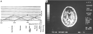
The first published explanation of the contrast seen in human brain MR images was that described by Godfrey Hounsfield during his Nobel Prize Lecture on 8 December 1979. Godfrey was best known for his work on computed tomography (CT) (1-4) but the final figure in his lecture (Figure 1A) related the amplitude of the signal seen on a display of an MR inversion recovery (IR) image of the brain of one of the authors (IRY) (Figure 1B), to values of T₁ of tissues and fluids including white and gray matter shown on the image (Figure 1A) (5). In this figure three functions are seen, one of which (the curve next to the numeral 2) shows the amplitude of the signal from white matter greater than that from gray matter, which is what is apparent on the image. It was Godfrey’s method of understanding the signal and contrast of MR images and was published before a single brain patient had been studied with MR imaging. However, Godfrey did not describe the mathematical function or functions linking the signal and contrast seen on the image to T₁ during his lecture, or in the patents and papers he subsequently filed or wrote on MR imaging.

Figure 1 Nobel Lecture JenyFig 19b (5) (A) and brain (B) obtained in Autumn 1979 at the CRL of EMI Ltd with subject “Ian”. Godfrey Hounsfield’s plot of signal Amplitude against log relaxation time T1 for tissues and fluids (A), and an IR image of Ian Young’s brain showing high signal in white matter and lower signal in gray matter. In (A) there are two continuous curves and two dashed curves. On the continuous curve close to the number 2, White Brain has a higher signal than Gray Brain which is how these tissues appear on the image (B). (Figure 1A is published by courtesy of the Nobel Foundation).

An MR imaging pulse sequence can be thought of in two parts, firstly a preparation component which modifies tissue or fluid magnetization using radiofrequency (rf) pulses (e.g., 90^o, 180^o) as well as gradients, and secondly an acquisition portion concerned with detecting signal from transverse magnetization and localizing this in space using gradients either in conjunction with, or without additional rf pulses. This creates image voxels. The signal magnitude and phase of a voxel seen on an image are directly related to the transverse magnetization detected during acquisition. Contrast is the difference, or the fractional difference in signal or phase between two voxels. Contrast can be intrinsic when it is related to a single tissue (e.g., normal or abnormal), or extrinsic when it involves two different tissues or fluids.

The key ideas necessary for frequency and phase encoding in the acquisition portion of MR sequences have been incorporated into the concept of k- space which deals with spatial localization, and relates the data collection part of the pulse sequence to the resulting image via inverse Fourier Transformation (6-8). K-space has proved to be a concept of fundamental importance for understanding signal localization and image contrast as well as generating new ideas for research.

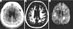
Understanding the preparation part of pulse sequences, as Godfrey sought to do in 1979, has been more complicated. By 1982, there were at least two types of MR image used in clinical practice (Figure 2), one employing the IR sequence in which differences in T₁ were the main source of contrast (as shown in Figure 2B), and the other using a spin echo (SE) sequence in which differences in T₂ were the main source of contrast as shown in Figure 2C (9). The two types of images appeared very different. There was no comparable phenomenon in CT at this time; essentially all unenhanced CT images appeared the same. It was necessary to distinguish the two types of MR image, and during 1983 the concept of weighting was used to do this (10,11). Images were described qualitatively as T₁- weighted or T₂-weighted when changes or differences in T₁ or T₂ were (respectively) thought to be the main source of contrast seen on them. The terms T₁ and T₂-weighted were also applied to the pulse sequences used to generate the images.

Figure 2 Multiple Sclerosis, 1982. CT (A), IR image (B) and SE image (C). The IR image (B) shows high gray white matter contrast with low signal lesions (e.g., arrows), while the SE image (C) shows little or no gray white matter contrast and lesions with high signal (e.g., arrows). The appearances of images (B) and (C) are quite different. IR, inversion recovery; SE, spin echo.

The terms T₁ and T₂-weighted were not included in the first edition of the Glossary of NMR Terms published by the American College of Radiology (ACR) Subcommittee on Nomenclature and Phantom Development in 1983 as they had only just come into use at this time (12). The Glossary became the accepted standard for MR nomenclature at MR meetings and for articles in journals on the subject (13,14).

Three years later in 1986, the ACR Subcommittee decided not to list the terms T₁-weighting and T₂- weighting in the second edition of the Glossary (15) on the grounds that they were “ambiguous”, “confusing”, and “implied that the dominant source of contrast was T₁ and T₂ when often this was not true” (16). Following this, some journals did not publish papers that used the terms T₁-weighted and T₂-weighted in compliance with the intention of the Glossary (17,18). However, during this time other articles were published using the terms (19,20), and both T₁ and T₂-weighting continued to be used in clinical practice since some method of relating the appearance of MR images to MR tissue (and fluid) properties such as T₁ and T₂ was necessary for image interpretation. This was because both the normal and pathologic appearances seen on MR images are understood in terms of the differences, or changes produced in these properties. The ACR subcommittee did not propose an alternative to the concept of weighting, or a refinement of it in order to resolve the problems associated with its use.

In spite of the reluctance to include them in 1986, the terms T₁-weighting and T₂-weighting were included in the third edition of the ACR Glossary published in 1991, and in subsequent editions published in 1995 and 2005 with the definitions unchanged from 1991Jeny (21-23). These are shown in Table 1 together with other definitions of T₁ and T₂- weighting (24,25).

However, the problems associated with use of the concept of weighting did not go away.

Some of these are illustrated in Figures 3-8:

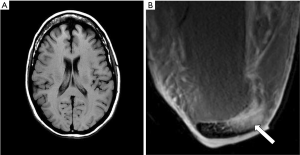
• Figure 3A shows a T₁-weighted image of the brain in which short T₁ tissues, such as fat and white matter have a high signal, and long T₁ CSF has a low signal in accordance with their T₁ values. When the same sequence is used to image the Achilles tendon in Figure 3B it is usually described as T₁-weighted, but the abnormal high signal in the tendon (arrow) is not due to a short T₁ from the presence of fat, hemorrhage or gadolinium, but is due to an increase in the T₂ of the tendon (e.g., from edema, tear or degeneration). These are very different explanations for the abnormality. The T₁-weighted sequence for the brain is T₂-weighted for the Achilles tendon, and the high signal within the tendon is due to an increase in T₂, not a decrease in T₁.
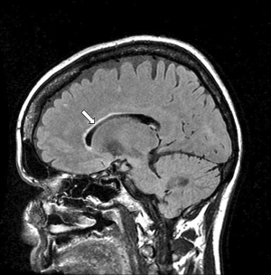
• The “T₂-FLAIR” (FLuid Attenuated IR) image shown in Figure 4 is highly T₂-weighted for the brain but simultaneously highly T₁-weighted for CSF. Thus, the principal source of contrast on the image varies depending on the tissue or fluid under consideration. In addition, the high contrast of the T₂ -FLAIR image relative to T₂-weighted SE images is achieved by doubling the TE of the T₂- FLAIR sequence, not using a TE between those of the tissues of interest (normal and abnormal brain) as recommended by the ACR in Table 1.
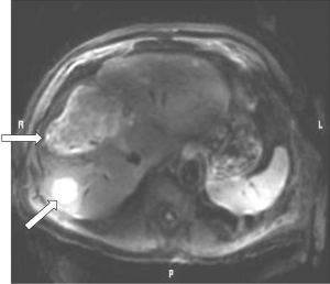
• Although the image in Figure 5 is described as “diffusion weighted” it is more T₂-weighted than diffusion weighted.
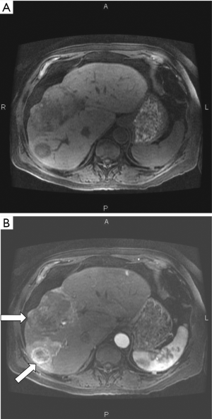
• It is generally recommended that high flip angles should be used to maximize T₁ contrast with spoiled gradient echo (SGE) sequences, but a low flip angle of 8° has been used to show the contrast enhancement with Gd-DPTA due to T₁ shortening seen in Figure 6B.
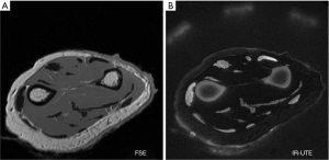
• It is generally stated that decreasing TE reduces T₂-weighting (Table 1). However, the ultrashort TE (UTE) image shown in Figure 7B has an extremely short nominal TE of 8µs but is highly T₂-weighted. In addition, the signals from tissues shown on this image decrease with increasing T₂, contrary to the definition of T₂-weighting included in Table 1 (25).
• It is not clear whether the Double Inversion Recovery (DIR) image shown in Figure 8 has twice the T₁-weighting of a conventional IR image, half of it, or differs in some other way.

Figure 3 Brain and Achilles tendon, both examined with the same T₁-weighted SE sequence. Transverse “T₁-weighted” SE images of the brain (A) and the Achilles tendon (B). The brain shows white matter with high signal, gray matter with intermediate signal and CSF with low signal in accordance with their T₁s and is T₁-weighted (A). In (B) the abnormal Achilles tendon is high signal (arrow). This is not because it has a short T₁ (e.g., due to hemorrhage, fat or contrast enhancement with Gd-DTPA), but because it has an increase in T₂ (e.g., due to edema or degeneration). For the Achilles tendon the sequence is T₂-weighted not T₁-weighted, and the high signal within it is due to an increase in T₂ not a decrease in T₁. SE, spin echo.

Figure 4 T₂-FLAIR image of the brain. The brain is heavily T₂-weighted and shows some anterior and superior periventricular high signal (arrow), but the CSF is heavily T₁-weighted.

Figure 5 Transverse image of the liver showing high signal tumors (arrows) obtained with a conventional “diffusion weighted” sequence with b=300 s/mm². The sequence is more T₂-weighted than diffusion weighted.

Figure 6 SGE images of the liver before (A) and after (B) administration of intravenous Gd-DTPA. Contrast enhancement is seen in the tumors in (B) (arrows) using a low flip angle of 8°, not a high flip angle. SGE, spoiled gradient echo.

Figure 7 Transverse FSE (A) and IR-ultrashort TE (IR-UTE) (B) images of the forearm. Cortical bone, aponeuroses and tendons are low signal in (A) and high signal in (B). The IR-UTE image (B) is highly T₂-weighted for cortical bone, tendons and aponeuroses in spite of its extremely short nominal TE of 8 µs. FSE, fast spin echo.

Figure 8 Double inversion recovery image of the brain showing gray matter alone with no signal from white matter or CSF. It is not clear whether it has more, or less T₁-weighting than a single IR image of the brain.

Table 1 ACR and other definitions of T₁ and T₂-weighting
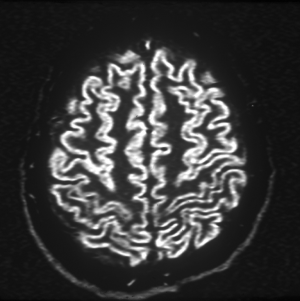
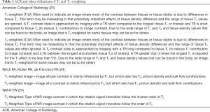
Full table

These problems, and numerous others like them, add an extra dimension of difficulty to the physics used to explain clinical MRI which is already complex.

Although comprehensive descriptions of MR imaging are available in the MR physics literature, they do not include mathematical definitions of weighting and the term is not even included in the indexes of the two of them (26,27), even though weighting is the concept most widely used in clinical practice for MR image interpretation.

The lack of a specific definition and the numerous inconsistencies and ambiguities associated with the use of the term weighting has meant that the concept has never gained the wide currency which that of k-space has.

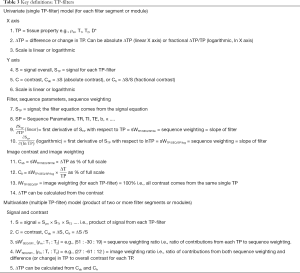
The general objective of this paper is shown in Table 2. This is to relate the MR properties of tissues and fluids shown in the left column to the signal and contrast of two or more voxels seen on an image shown in the right column, via a knowledge of the pulse sequences and their sequence parameters used to image the tissues and fluids which are shown in the central column.

Table 2 Tissue and fluid properties, pulse sequences and sequence parameters, and image features
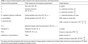
Full table

The specific objectives are:

• To describe mathematical functions which relate tissue properties (TPs) to the signal and contrast seen on MR images as originally envisaged by Godfrey Hounsfield.
• To convert conventional qualitative weighting into quantitative forms of weighting.
• To use these approaches to explain problems that arise from the use of the qualitative approach to weighting.
• To provide a basis for relating the preparation component of pulse sequences to voxel signal and contrast seen on images that is complementary to the use of k-space to relate the signal acquisition of pulse sequences to the spatial properties of MR images and their global contrast.

Tissue properties (TPs)

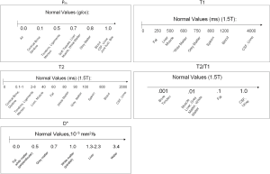
As an initial step it is helpful to review some features of the normal values of tissue and fluid properties (e.g., ρ_m, T₁, T₂, $\frac{{\text{T}}_{\text{2}}}{{\text{T}}_{\text{1}}}$ and D*) that are frequently encountered in clinical practice (Figure 9). Normal values of some of these properties cover at least three orders of magnitude and so it is helpful to display them on a logarithmic scale as Godfrey Hounsfield did in Figure 1A. This compresses the range of values and lends itself to the use of fractional differences such as $\frac{\Delta {\rho }_{\text{m}}}{{\rho }_{\text{m}}}$, $\frac{\Delta T_{\text{1}}}{T_{\text{1}}}$ and $\frac{\Delta T_{\text{2}}}{T_{\text{2}}}$ in the form of fractions or percentages to describe changes, since a small change on a logarithmic scale $\Delta I\text{n}x=\frac{\Delta x}{x}$.

Figure 9 Values of ρ_m, T₁, T₂, T₂/T₁ and D*.

Mobile proton density (ρ_m)

ρ_m means the density of protons (or spin density) with T₂s long enough to be detected with MR systems. In the past the lowest level of detectability for clinical systems corresponded to a T₂ of about 10 ms. Now the minimum value of T₂ is probably about 0.1 ms using ultrashort echo time (UTE) pulse sequences with (nominal) TEs as short as 8 µs. The ρ_m of bone is about 15–20%, meniscus and cartilage about 50–70%, soft tissues about 70–90% and relatively pure fluids very close to 100%. The difference (about 10–20%) in ρ_m between gray and white matter is because white matter contains more immobile or bound (MR “invisible”) protons with ultrashort T₂s (0.1–1 ms) associated with myelin. The chemical proton densities (which includes all protons) of gray and white matter are similar.

T₁

The pattern for mean T₁s generally follows that for ρ_m with the shortest mean T₁s those of cortical bone (130–200 ms at 1.5T), and the longest those of CSF and other fluids (about 4,000 ms). Fat has a short T1 (e.g., 250 ms at 1.5T). Contrast enhanced blood may have a T₁ as short as 15–20 ms (28). Values of T₁ tend to increase with static field strength (B₀) approximately to the power of 0.3 or 0.4, while T₂ values tend to decrease with increasing B₀, but to a lesser extent (29,30).

T₂ and T₂/T₁

In general terms, the pattern of mean T₂s follows that for ρ_m and T₁, with T₂ shortest for cortical bone (0.3–0.5 ms) (31), followed by tendons, ligaments and menisci (1–8 ms) (32), soft tissues, and fluids. Fat is an exception since it has a short T₁ and a long T₂. Because of issues associated with measurement, widely varying values are quoted for the T₂s of fluids such as CSF extending from 2,000–3,000 ms down to about 200–300 ms. Values for T₂ of some tissues and fluids and the ratio of $\frac{{\text{T}}_{\text{2}}}{{\text{T}}_{\text{1}}}$ are shown for some common tissues in Figure 9 (at 1.5T). For T₂/T₁ there are four groups of tissues and fluids of interest, namely bone and tendon (≈0.001), water containing soft tissues (≈0.01), fat (≈0.1) and fluids (≈1).

D*, the apparent diffusion coefficient

Mean values of D* follow the same general pattern but with the important addition of anisotropy, with white matter having a higher D* when its fibers are parallel to the gradient field than when its fibers are perpendicular to this field.

Susceptibility (χ)

Susceptibility can be divided into large scale (bulk) and microscopic, and applies to tissues, fluids and materials inside the body. The basic classification is by the change in field produced by the substance and is divided into diamagnetic (slight decrease), paramagnetic (slight increase), superparamagnetic (large increase), and ferromagnetic (large and persistent increase). On the large scale, susceptibilities range from titanium (1.8×10⁻⁴), “nonmagnetic” stainless steel (Jeny10^-1), magnetic stainless steel (10³), and pure iron (10⁵). Most soft tissues are in the much smaller microscopic range of −7 to −11×10⁻⁶. Susceptibility is also dependent on geometric factors including the orientation of ordered fibers to the main magnetic field. Fibers may show a sin²Θ dependence where Θ is the orientation of the fibers to B_0. Modelling of voxels as individual dipoles produces more accurate differentiation between tissue susceptibility, geometric and dipolar effects.

Chemical shift (δ)

Triglyceride containing tissues of the body include subcutaneous and visceral fat, yellow bone marrow, red bone marrow, liver, and muscle. The fat has multiple spectral peaks, each with different resonant frequencies (and thus δs), T₁s and T₂s. The largest peak is from –CH₂ and is usually located at −3.3 ppm lower than water. In addition, metabolically active brown adipose tissue with about 30–70% triglyceride and 30–70% water may be detected mainly in the neck, mediastinum and upper abdomen.

Although TPs are usually thought of as inherent, and independent of measurement technique, frequently they are described in qualified terms e.g., mobile, observed, measured, or apparent (e.g., ρ_m, T_1obs, T₂*, D*) where the value of the property is affected by additional factors [e.g., MR machine limitations, susceptibility, chemical shift differences, magnetization transfer (MT)], measurement errors and the use of simplified models.

In addition, quite frequently what is observed is populations of protons with different MR properties within a voxel. The observed signal from a voxel may reflect the complex sum of the signals from two or more tissue or fluid components including effects due to differences in resonant frequency (due to susceptibility and/or chemical shift) between different components.

Normal tissues are usually described as showing differences, while abnormal or acquired differences from normal are usually described as changes.

Further details on tissues are included in later sections. More detailed values of tissue properties are available in the MR imaging literature. There are also other tissue and fluid properties of importance including shear stiffness, conductivity, and permittivity which are not dealt with here for reasons of space. The term “tissue” is subsequently used in this paper to include fluids unless otherwise specified.

Changes in TPs in disease

Changes in TPs in disease are the subject of an extensive literature and are only briefly outlined here. The most common change in MR TPs in disease is an increase in ρ_m, T_1, T₂ (and often D*) with the fractional change in the latter three properties usually being much greater than that in ρ_m. This is typically seen in acute infection, acute inflammation, edema, and many tumors. Reductions in these TPs are less commonly seen in disease but occur in important conditions, including some stages of hemorrhage (T₁, T₂), acute cerebral infarction (D*) and tumors (D*) [for example (33)]. A reduction in tissue T₁, T₂ and T₂* may also be seen with accumulation of paramagnetic species such as iron.

Increased fat content is seen in liver disease either primarily or secondarily. Tissue magnetic susceptibility typically increases with increased iron content and accumulation of some hemoglobin breakdown products, and decreases with calcification. Other changes in TPs in disease are mentioned in later sections under relevant headings.

The SE sequence (univariate, single TP-filter model)

The SE pulse sequence as three separate TP-filters

The SE sequence consists of an initial 90^o pulse, followed by a 180^o refocusing pulse and a data acquisition centered at time TE after the 90^o pulse for conventional SE sequences, and at TE effective (TE_eff) for fast SE sequences, with the cycle repeated after repetition time TR. It is common to explain contrast in this sequence in terms of tissue longitudinal magnetization followed by transverse magnetization on the Y axis both plotted against time on the X axis with longitudinal magnetization becoming transverse when the 90^o pulse is applied (Figure 10). Contrast is represented at time TE by the difference in transverse magnetization along the Y axis, and hence signal difference between the two curves for tissues P and Q as shown in Figure 10. While this approach is useful for explaining signal and contrast, it is less helpful for understanding the weighting of the sequence and the resulting image.

Figure 10 Composite M_z/M_xy vs time diagram for the SE sequence for two tissues P and Q. This shows recovery of the longitudinal magnetization (M_z) for time TR, followed by decay of the transverse magnetization (M_xy) for time TE after the 90° pulse of the SE sequence. Signal is proportional to M_xy at time TE. The contrast between the two tissues is proportional to the difference between the two curves (vertical line) at time TE. SE, spin echo.

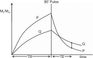
From the Bloch equations the simplified signal equation for SE or fast SE (FSE) sequences is given by:

where K is a scaling function and S is voxel signal (i.e., magnitude). The equation can be written:

with

${\text{S}}_{{\text{ρ}}_{\text{m}}}$, ${\text{S}}_{{\text{T}}_{\text{1}}}$, ${\text{S}}_{{\text{T}}_{\text{2}}}$ and are the normalized signals for the separate segments of the equation for each of ρ_m, T₁ and T₂. T₁ is scaled relative to the sequence parameter TR, and T₂ is scaled relative to the sequence parameter TE (or TE_eff). In the above equation, and subsequent text, TE is used to represent either TE or TE_eff. A list of key definitions is included in Table 3.

Table 3 Key definitions: TP-filters
Full table

If instead of plotting magnetization (and potential signal) against time as in Figure 10, the voxel signal S is plotted against the natural logarithm of T₁ (lnT₁), and against lnT₂, for the fixed times of the pulse sequence TR and TE, the curves shown in Figure 11 result. The signal equations of these curves are of the form $\text{y}=1-{\text{e}}^{-\frac{\text{1}}{\text{x}}}$ and $\text{y}={\text{e}}^{-\frac{\text{1}}{\text{x}}}$. This is because the variables are the T₁s and T₂s of the different tissues seen on the respective images, rather than time, which has the constant values TR and TE for the latter two segments of the SE sequence. The more familiar exponential equations y = 1−e^−x, and y = e^−x describe the recovery of longitudinal magnetization, and the decay of transverse magnetization against time respectively as illustrated in Figure 10.

Figure 11 SE T₁-filter (A) and T₂-filter (B). Plot of against lnT₁ (A), and against lnT₂ (B) for given values of TR (A) and TE (B). The curves have the appearance of a low pass filter (A), and a high pass filter (B). Both filters are sigmoid shaped with high and low signal plateaus, as well as sloping regions or transition bands between them. Short T₁ values give a high signal in (A), and long T₂ values give a high signal in (B). SE, spin echo.

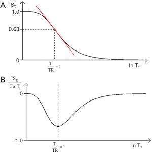
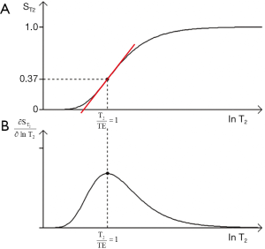
The curves shown in Figure 11 have the shapes of a low pass filter (low/short values of T₁ “pass” i.e., are not reduced, whereas high/long values of T₁ are reduced or stopped) in Figure 11A, and a high pass filter (high/long values of T₂ “pass”, and low/short values of T₂ are reduced or stopped) in Figure 11B. Increase in TR shifts the T₁-filter in Figure 11A to the right (Figure 12A). Increase in TE also shifts the T₂-filter shown in Figure 12B to the right. The two filters shown have low pass (or stop) bands and high pass bands as well as transition bands between the two. The transition bands are often the part of the filter of most clinical interest. The term “filter” is used in many different contexts, but the sense used here is analogous to that employed in electronics to describe the blocking or passing of electrical signals depending on their frequencies in resistive-inductive-capacitative (RLC) circuits. The filters in this paper are designated by the TP, or other quantity along their X axis as well as by functional or descriptive terms (e.g., high/low pass, notch).

Figure 12 SE T₁-filter (A) and SE T₂-filter (B). With the T₁-filter (A) increase in TR shifts the curve to the right. With the T₂-filter (B) increase in TE also shifts the curve to the right. SE, spin echo.

The signal intensities shown on the T₁-filter for fat (F), white matter (W), gray matter (G) and CSF in Figure 13A correspond with the signal (brightness) seen on the T₁-weighted SE image shown in Figure 13B. The signal intensities shown on the T₂-filter for white matter (W), gray matter (G) and CSF shown in Figure 14A correspond with the signal seen on the T₂-weighted SE image shown in Figure 14B.

Figure 13 SE T₁-filter (A) and corresponding T₁-weighted image of the brain (B). The signal intensities of fat (F), white matter (W), gray matter (G) and CSF shown on the T₁-filter (A) correspond with the signal (brightness) seen in these tissues and CSF on the image (B).

Figure 14 SE T₂-filter (A) and corresponding T₂-weighted image of the brain (B). The signal intensities of white matter (W), gray matter (G) and CSF shown on the T₂-filter (A) correspond with the signal (brightness) seen in the tissues and CSF on the image (B).

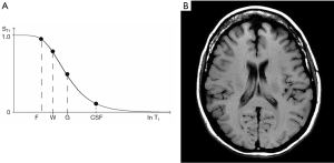
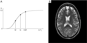
Figure 15 shows the SE T₁-filter for two tissues P and Q. Increase in T₁ from P to Q along the X axis produces negative contrast from P to Q along the Y axis as a function of the slope of the curve shown in red which is the sequence weighting. Figure 15 also shows the difference in signal ΔS_T1 (or absolute contrast, C_ab) between two voxels that results from a difference in T₁ of $\Delta I{\text{n T}}_1=\frac{\Delta {\text{T}}_1}{{\text{T}}_1}$ between two tissues P and Q, for small ∆s. Positive change in ΔlnT₁ from P to Q along the X axis results in negative contrast from P to Q along the Y axis. The value of C_ab = ΔS_T1 is given by the slope of the filter (m) multiplied by the fractional difference ∆lnT₁ (since Δy = mΔx).

Figure 15 SE T₁-filter. Relationship between change in lnT₁ (ΔlnT₁ = ΔT₁/T₁ for small Δ) and change in signal (contrast) $\Delta S_{T_1}$. The (positive) difference ΔlnT₁ from P to Q produces a (negative) change in signal $\Delta S_{T_1}$ from P to Q along the Y axis. This is in a region where the curve is steeply sloping. Difference or change in ΔlnT₁ would produce little or no signal difference (or contrast) in regions corresponding to either of the high or low signal plateaus of the curve. The slope of the curve between P and Q shown in red is the sequence weighting for this T₁-filter. It is negative.

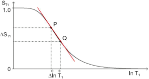
In addition to the central highly sloping region, the curve has both high and low signal plateaus where its slope is much lower. Changes or differences in ∆lnT₁ along the X axis in these regions produce much less change in signal than in the central region, and therefore less contrast.

The sequence weighting sW_T1/_SE is the slope of the filter, m. It is the contribution the sequence makes to contrast. In Figure 16 it is the first partial derivative of the T₁-filter ($\frac{\partial S_{T_1}}{\partial \ln T_1}$) and is shown in Figure 16B. It can be calculated using the identity $\frac{dy}{d(\ln x)}=x\frac{dy}{dx}$. The slope of the derivative is zero or negative and reaches a minimum (maximum negative value) at the point where $\frac{{\text{T}}_1}{\text{T}R}=1$ i.e., T₁=TR. The slope of the curve at this point is shown in red in Figure 16A. This is the point of maximum (negative) sequence weighting. It is achieved at 63% of the maximum signal. The partial derivative seen in Figure 16B extends both to the right and to the left of this point showing that there is significant weighting away from the maximum value, and that this is greater $\frac{{\text{T}}_1}{\text{T}R}$ for multiples of on the right than for the corresponding fractions of $\frac{{\text{T}}_1}{\text{T}R}$ on the left.

Figure 16 SE T₁-filter (A) and its first partial derivative (B). Plot of ${\text{S}}_{{\text{T}}_{\text{1}}}$ against lnT₁ (A), and $\frac{\partial {\text{S}}_{{\text{T}}_{\text{1}}}}{\partial {\text{In T}}_1}$ against lnT₁ (B). The slope of filter is shown in red (A) and is shown in (B) where it is negative or zero. This is the sequence weighting for the T₁-filter. The slope reaches a maximum negative value at $\frac{{\text{T}}_1}{\text{TR}}=1$. This is at (1‒e⁻¹) =0.63=63% of the maximum signal shown in (A).

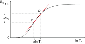
The same general principles apply to the T₂-filter except that it has a positive slope (Figure 17). The positive change ∆lnT₂ from P to Q along the X axis produces a marked positive change in signal ∆S_T2 (or absolute contrast C_ab) from P to Q when this corresponds with a highly sloping region of the T₂-filter. The slope between P and Q is shown in red. Less change in signal is produced by a change ∆lnT₂ in regions corresponding to the high and low signal plateaus. The slope of the T₂-filter, $\frac{\partial S_{T_2}}{\partial \ln T_2}$ is the sequence weighting for this filter and is shown in red in Figure 18A at its maximum. The slope of the whole filter is shown in Figure 18B. This has a maximum positive value where $\frac{\text{TE}}{{\text{T}}_2}\text{=}1$, i.e., T₂ = TE using a lnX scale. This is achieved at 37% of the maximum signal.

Figure 17 SE T₂-filter. Plot of ${\text{S}}_{{\text{T}}_{\text{2}}}$ against lnT₂ for two tissues, P and Q. The (positive) difference ΔlnT₂ from P and Q along the X axis produces a (positive) difference in signal (contrast) $\Delta {\text{S}}_{{\text{T}}_{\text{2}}}$ along the Y axis where it is opposite a steeply sloping region of the curve. Little or no contrast would be produced by ΔlnT₂ if it was opposite either the upper or the lower plateaus of the curve. The slope of the T₂-filter between P and Q shown in red is the sequence weighting which is positive.

Figure 18 SE T₂-filter (A) and its first partial derivative (B). Plot of ${\text{S}}_{{\text{T}}_{\text{2}}}$ against lnT₂ (A), and $\frac{\partial {\text{S}}_{{\text{T}}_{\text{2}}}}{\partial {\text{In T}}_2}$ against lnT₂ (B). The slope of curve (e.g., red line) in (A) is shown in (B) where it is positive or zero. It is the sequence T₂-weighting. It goes through a maximum at $\frac{{\text{T}}_2}{\text{TR}}=1$ where the signal level is 0.37=37% of the maximum shown in (A).

Absolute contrast (C_ab) and fractional contrast (C_fr)

So far only absolute contrast (C_ab= ΔS) has been considered, but fractional contrast (or a variant of this) between two voxels ($C_{\text{fr}}=\frac{\Delta \text{S}}{S}$ or groups of similar voxels) is also important in MR imaging. To obtain C_fr the partial derivatives of the TP-filters shown in Eq. [2] are divided by S_ρm, S_T1, and S_T2 respectively to obtain normalized forms of sequence weighting for each of the three TP-filters i.e.:

This is only valid if, and are not low or zero. The prefix s used in Eq. [4] designates sequence weighting. The subscripts are shown here in the order TP /sequence/type of contrast. More detailed notation for weighting is provided in Table 4. Weighting only needs to be specified to the degree necessary for the purpose at hand.

Table 4 Notation for weighting
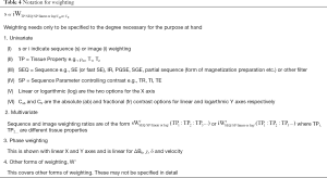
Full table

Contrast is sequence weighting multiplied by fractional change in TP so C_ab for each TP-filter is:

and fractional contrast (C_fr) for each TP-filter is:

On the Y axis of the TP-filters, C_ab is shown on a linear scale, and C_fr is shown on a logarithmic scale.

Large differences or changes in tissue properties

So far we have only dealt with small changes in tissue properties and used partial derivatives to calculate sequence weighting and combined this with the fractional change in TP to give contrast for each TP.

However, there may also be large differences or changes in tissue properties. In this case we can determine the sequence weighting for two tissues, P and Q, as the mean slope of the filter m. For the particular case of a T₁-filter using a logarithmic X axis:

The contrast m is then multiplied by the TP difference to give the contrast.

It is possible to determine the value of TR to maximize m, and hence the sequence weighting for the values of T₁ at P and Q using numerical methods based on the sequence signal equation. Pelc showed that the large difference (discrete approach) and the use of derivatives (the continuous approach) showed only small disagreement and converged for smaller difference in T₁ in his study of the SGE sequence (34).

The ρ_m-filter

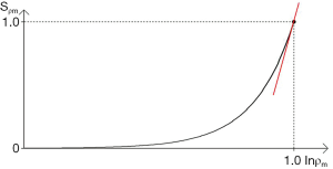
The final filter for the SE sequence is the ρ_m-filter. If the X axis was linear it would be a straight line, but since a logarithmic X axis is being used, it is a positive exponential (Figure 19). The maximum slope is shown in red.

Figure 19 Plot of ${\text{S}}_{{\text{ρ}}_{\text{m}}}$ against lnρ_m. The logarithmic scale compresses high values of ρ_m and so the curve is steeper on the right. The slope of the curve is the ρ_m sequence weighting (e.g., red line). It is highly positive at the maximum of ρ_m (1.0).

The univariate (single TP-filter) model

The univariate model only deals with difference or change in one filter ${\text{S}}_{{\text{ρ}}_{\text{m}}}$, ${\text{S}}_{{\text{T}}_{\text{1}}}$ or ${\text{S}}_{{\text{T}}_{\text{2}}}$ at a time, with the other two TP-filters assumed to be, or made constant.

For change in the T₁-filter alone we want $S_{T_2}=e^{-\frac{TE}{T_2}}$ to be constant. If $\frac{TE}{T_2}$ is low as with short values of TE and long values of T₂$S_{T_2}$ is nearly equal to 1 on the right side of the SE T₂ filter (Figure 17) and is constant, or nearly constant. If in addition Δρ_m = 0, so that only T₁ changes, we can use the univariate model for T₁.

If we are interested in change in T₂ alone we want S_T1 to be constant and ≈ 1 (i.e., TR/T₁ high, TR long and T₁ short so e^−TR/T1 ≈ 0) as well as $\frac{\Delta {\rho }_{\text{m}}}{{\rho }_{\text{m}}}\text{=}0$. Then with only $S_{T_2}$ changing, we can use the univariate model for T₂ changes. Pulse sequences are frequently designed to minimize the weighting of one of T₁ or T₂ and maximize the other, and quite often $\frac{\Delta {\rho }_{\text{m}}}{{\rho }_{\text{m}}}$ is small or zero. In these circumstances the univariate model can provide a useful way of understanding the signal and contrast produced by the SE sequence.

Summary of the univariate model of the SE sequence

• The univariate model considers each segment of the SE signal equation separately, and defines respectively an exponential, a low pass and a high pass TP- filter for ρ_m, T₁, and T₂. As illustrated, here it uses natural logarithms or scaled logs for the TP values but linear TP values can also be used.
• The first partial derivative of the TP-filter equation is the slope of the filter which is its sequence weighting.
• For T₁ and T₂, the slope of the filter can be maximized using the second derivative of the T₁ or T₂-filter to determine a point of inflexion. This gives the values of TR or TE for maximum sequence weighting of TR=T₁ and TE=T₂ respectively using a lnX axis. For a linear X axis the corresponding values are TR = 2T₁ and TE = 2T₂.
• The location of the filters relative to the X axis can be changed by varying the sequence parameters TR and TE. The location of the T₁ filter along the X axis can be determined by noting that its sequence weighting is maximized when TR = T₁ where there is 63% of the signal. The T₂-filter location can be determined by noting that its sequence weighting is maximized at TE = T₂ with 37% of the signal.
• The C_ab of each TP-filter is the first partial derivative of the filter (its sequence weighting) multiplied by the change in TP.
• The same calculation can be performed for fractional contrast C_fr which is the first partial derivative of the filter multiplied by the change in TP divided by the filter signal, providing that signal levels are not low or zero.
• For large changes in tissue properties, the mean slope of the TP-filter can be calculated to provide a measure of the sequence weighting for two different tissues rather than the first partial derivative.
• The model distinguishes between sequence and image weighting.
• The image weighting (i.e., the proportion of the contrast C_ab or C_fr, whether positive or negative, attributable to each TP) is ±100% for each ρ_m, T₁, and T₂ filter.
• The univariate model can be appropriate clinically in specific situations where Δρ_m is low or zero, and T_2-weighting has been minimized so that only changes in T₁ described by the T₁-filter are considered (or vice versa for T₂-weighting). T₁ and T₂ dependence can both be concurrently minimized in order to assess ρ_m effects.
• Conventional weighting is qualitative. It is also univariate since it designates a single TP as the principle source of contrast.
• The univariate TP-filter model provides the mathematical formalism for converting conventional univariate qualitative weighting into quantitative univariative weighting for each TP. This results in a variety of new insights which are not apparent using qualitative weighting.

The SE sequence (multivariate, three TP-filter model)

The multivariate model

In the previous section we dealt with the situation where only one of ${\text{S}}_{{\text{ρ}}_{\text{m}}}$, ${\text{S}}_{{\text{T}}_{\text{1}}}$ or ${\text{S}}_{{\text{T}}_{\text{2}}}$ varied at a time. However, the more general situation is where all three tissue properties ρ_m, T₁, and T₂ differ or change. This is treated in the same way as for the univariate model for each TP-filter, but instead of deriving functions for change in each TP alone, weighting ratios are used. These are the ratio of the individual TP weightings to the sum of the magnitudes of all the TP weightings expressed as a percentage. This measure includes all three properties and quantifies the contribution each TP makes to overall sequence and image weighting (see Table 3 for definitions).

We can take first derivatives of Eqs. [2] and [3] and use a lnX scale so for the whole sequence C_ab= ΔS is given by:

Normalizing this, providing that none of S, ${\text{S}}_{{\text{ρ}}_{\text{m}}}$, ${\text{S}}_{{\text{T}}_{\text{1}}}$ or ${\text{S}}_{{\text{T}}_{\text{2}}}$ are low or zero, gives:

For each TP the initial term on the right is the first partial derivative of the filter divided by the filter itself. This is the normalized first partial derivative for the TP. It is multiplied by the fractional difference in TP in Eqs. [8] and [9].

Using Eqs. [9] and [3] we can evaluate the normalized partial derivatives and define the sequence weighting ratio $s{W}_{SE}^{\text{r}}$ as the relative contribution of each of the tissue properties to the overall sequence weighting (see Table 4) where:

For the corresponding image weighting ratio $i{W}_{SE}^{\text{r}}({\rho }_m:T_1:T_2)$ we multiply the normalized partial derivative for each TP (as in the sW^r) by the relevant fractional change in TP $\frac{\Delta {\rho }_{\text{m}}}{{\rho }_{\text{m}}}$, $\frac{\Delta T_{\text{1}}}{T_{\text{1}}}$ and $\frac{\Delta T_{\text{2}}}{T_{\text{2}}}$ so that:

The image weighting ratio is the ratio of the total contributions (from the sequence weighting multiplied by the change in TP) made by each TP to the overall contrast. Within the proscribed limits (no low or zero signals for S, S_ρm, S_T1 or S_T2) it describes the contribution of each TP to the image weighting in quantitative terms. For the non-zero values described previously the weighting ratios are the same for each type of contrast, whether absolute (C_ab) or fractional (C_fr).

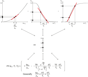
The contribution of all TP filters to image weighting is shown in Figure 20. The fractional difference in each TP $\frac{\Delta {\rho }_{\text{m}}}{{\rho }_{\text{m}}}$, $\frac{\Delta T_{\text{1}}}{T_{\text{1}}}$ and $\frac{\Delta T_{\text{2}}}{T_{\text{2}}}$ is multiplied by the slope of each filter (its sequence weighting) to give the difference in signal between two tissues or fluids P and Q (or the contrast $\Delta {\text{S}}_{{\text{ρ}}_{\text{m}}}$, $\Delta {\text{S}}_{{\text{T}}_{\text{1}}}$ and $\Delta {\text{S}}_{{\text{T}}_{\text{2}}}$ produced by each TP). Signals from each TP filter are multiplied together to give the overall signals for P and Q as shown at the center of the figure. The difference, or contrast between them is also shown. The image weighting ratio $i{W}_{SE}^{\text{r}}({\rho }_m:T_1:T_2)$ can be calculated from the normalized first partial derivatives (i.e., the sequence weightings) multiplied by the fractional differences in tissue properties as shown in the lower part of Figure 20.

Figure 20 SE sequence. Image signal, contrast and weighting for two tissues P and Q. The diagram shows how the fractional differences in each tissue property $\frac{\Delta \text{ρm}}{\text{ρm}}$, $\frac{\Delta {\text{T}}_1}{{\text{T}}_1}$ and $\frac{\Delta {\text{T}}_2}{{\text{T}}_2}$ are multiplied by the slopes of each filter in turn (${\text{S}}_{{\text{ρ}}_{\text{m}}}$, ${\text{S}}_{{\text{T}}_{\text{1}}}$, ${\text{S}}_{{\text{T}}_{\text{2}}}$) to give the signals for P and Q along the respective ${\text{S}}_{{\text{ρ}}_{\text{m}}}$, ${\text{S}}_{{\text{T}}_{\text{1}}}$, ${\text{S}}_{{\text{T}}_{\text{2}}}$ Y axes in the top row. These signals are then multiplied together to give the overall signals for P and Q and contrast (difference in signal) between them along the Y axis showing S in the center of the image. The corresponding calculations for the image weighting ratio ${\text{iW}}_{\text{SE}}^{\text{r}}\left({\text{ρ}}_{\text{m}}{\text{:T}}_{\text{1}}{\text{:T}}_{\text{2}}\right)$ are shown below, where each normalised partial derivative is multiplied by the corresponding fractional change in tissue property to give the contributions of each tissue property to the contrast between P and Q. The signals from ${\text{S}}_{{\text{ρ}}_{\text{m}}}$, ${\text{S}}_{{\text{T}}_{\text{1}}}$, ${\text{S}}_{{\text{T}}_{\text{2}}}$ are multiplied together to give the overall signal S, and contrast between P and Q along the Y axis shown at the center of the image.

A worked example

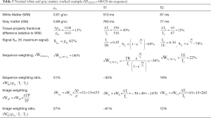
Table 5 shows a worked example for a SE sequence (SE_TR/TE = 600/20 ms) based on data for white and gray matter of the brain for a T₁-weighted image obtained at 1.5T from Hendrick (35). Normalizing by the sum of the magnitudes of the signals and using percentages, the sequence weighting ratio $\text{s}{W}_{SE}^{\text{r}}({\rho }_m:T_1:T_2)$ is (51:−30:19). In qualitative terms the sequence would be described as ρ_m-weighted (since ρ_m is the greatest source of contrast), but the image weighting ratio $i{W}_{SE}^{\text{r}}({\rho }_m:T_1:T_2)$, is (27: −61:12). This shows that the image would be described as T₁-weighted using the qualitative approach to weighting of naming the sequence by the TP which is the main source of contrast. Thus, in qualitative weighting terms, a ρ_m-weighted sequence has been used to produce a T₁-weighted image. The greater ρ_m-weighting of the sequence is overcome by the greater fractional difference in T₁ to produce the dominant T₁-weighting of the image.

Table 5 Normal white and gray matter, worked example (SE_TR/TE = 600/20 ms sequence)
Full table

Figure 3 shows a T₁-weighted SE sequence imaging brain (A) and Achilles tendon (B). Using the same values for the sequence parameters, but assuming a T₁ of 350 ms and T₂ of 2 ms for normal Achilles tendon the is $\text{s}{W}_{SE}^{\text{r}}({\rho }_m:T_1:T_2)$ (26:−9:65). In qualitative terms this shows that the sequence which is ρ_m-weighted for the brain is heavily T₂-weighted for the Achilles tendon.

Summary of the multivariate model of the SE sequence

• The multivariate SE model combines the filters for the three TP-filters ρ_m, T₁, and T₂ to give overall absolute or fractional contrast.
• The ratio of the contributions of the sequence tissue properties to the overall contrast is the sequence weighting ratio, $\text{s}{W}_{SE}^{\text{r}}({\rho }_m:T_1:T_2)$
• The sequence contributions are multiplied by the respective fractional differences or changes in tissue properties to provide the image weighting ratio, $i{W}_{SE}^{\text{r}}({\rho }_m:T_1:T_2)$
• Changes in the sequence parameters TR, and TE vary the weighting ratios.
• The sequence and image ratios are the same for C_ab and C_fr.
• Mean slopes can be used for large differences or changes in tissue properties.
• The multivariate model is generally applicable in clinical practice apart from situations where signals are low or zero.
• There is no equivalent way of describing multivariate weighting using the conventional qualitative approach to weighting which is univariate.

TP-filter diagrams for the SE sequence and other sequences are included at the end of the text of this paper. TP-filter equations and derivatives for the SE and other sequences are also included at the end of the text of this paper.

The IR sequence (TP-filter)

The IR sequence has an additional T₁-filter to that of the SE sequence giving a total of four filters. The second T₁-filter is controlled by the inversion time (TI) following the initial inversion pulse. If TR ≥ than the longest tissue (or fluid) T₁, the first T₁-filter (which is the same as for the SE sequence) allows virtually full recovery of all tissue longitudinal magnetization, and the overall signal is very largely, or wholly determined by the second (inversion) T₁-filter for which the signal equation is:

where TI is the inversion time. (The two T₁-filters can also be combined if necessary.) The ρ_m and T₂-filters are the same as for the SE sequence.

The long TR IR sequence (with a single inversion)

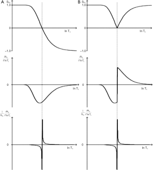
In this section the common long TR version of the IR sequence (with a single inversion) is considered. The T₁-filter for this sequence (Figure 21A) has twice the signal range (i.e., from +1 to –1) and twice the slope compared with the T₁-filter of the SE sequence. It also passes through zero with a null point where $1-2e^{-\frac{TI}{T_1}}=0$, and TI =0.69 T₁. Contrast is maximized on a natural log X axis scale where TI = T₁ and on a linear X axis scale where TI = 2T₁. This is achieved at 26% of the maximum signal. IR images can be reconstructed in either phase-sensitive (Figure 21A) or magnitude form where the negative signal shown in the Y axis beyond the null point is reflected across the X axis to become positive (Figure 21B). The slope of the filter at maximum sequence weighting is shown in red.

Figure 21 Long TR IR (single inversion) sequence T1-filters with phase sensitive (A), and magnitude (B) reconstruction. The curve in (A) has high and low signal plateaus with a sloping region between them. It has twice the range (+1 to −1), and twice the slope of the corresponding SE T₁-filter. The curve in (B) is the same as that in (A) up to the zero signal, or the null point. Beyond this the curve in (B) is a mirror reflection across the X (lnT₁) axis of the curve in (A). The slope of the filter is maximal at T₁ = TI (red lines) and this corresponds to a signal level of 0.26=26%.

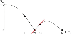
We can illustrate the three main classes of this form of the long TR IR sequence (36) by starting with a short TI and increasing TI (which displaces the curve to the right) using white (W) and gray (G) matter as fixed points of reference. In Figure 22A a short TI IR (STIR) sequence is shown with W matter signal less than that of G matter. In Figure 22B an intermediate TI sequence is shown with W matter signal greater than that of G matter, and in Figure 22C a long TI sequence, including the T₂-FLAIR sequence, is shown with both W and G matter high signal, with the signal from W matter slightly higher than that from G matter. The slopes of the curves which are their sequence weightings are shown in red. There is a similarity between Godfrey Hounsfield’s figure for the IR sequence (Figure 1A) and Figure 22.

Figure 22 T₁-filters for the long TR IR (single inversion) sequence. Plots of against lnT₁ are shown for a short TI (A), an intermediate TI (B), and a long TI (C). The positions of white matter (W) and gray matter (G) of the brain are shown along the X axis in (A), (B) and (C). In (A) (the STIR sequence), the signal from white matter is lower than that from gray matter. In (B) (the intermediate TI sequence) the filter is shifted to the right and the signal from white matter is higher than that from gray matter, and in (C) the long TI (e.g., T₂-FLAIR sequence) the filter is displaced further to the right and the signal from white matter is slightly higher than that from gray matter. The sequence weighting (red lines) is highly positive in (A), highly negative in (B) and slightly negative in (C). (A), (B) and (C) are the three main classes of the long TR IR sequence.

In the multivariate approach the positive contrast of the STIR sequence T₁ segment using magnitude reconstruction is combined with the positive contrast of the ρ_m and T₂ filters to give synergistic positive contrast when there is an increase in all three tissue properties ∆ρ_m, ΔT₁ and ΔT₂ in disease. With the intermediate TI sequence there is a high negative T₁ contrast. TE is usually reduced to minimize the opposed T₂ contrast. With the T₂-FLAIR sequence the slightly greater signal from white matter compared with gray matter (negative contrast) counters the opposed positive contrast from ρ_m, giving a net low contrast background between white and gray matter for the brain against which high signal lesions produced by the heavy positive T₂-weighting of the sequence and increase in T₂ of lesions can be seen. Although the T₂-FLAIR sequence has heavy T₂-weighting for the brain, it also often has 5–20% opposed T₁-weighting for this tissue. It also has very heavy negative T₁-weighting for CSF (i.e., the filter has a steep negative slope for values of T₁ just less than the T₁ of CSF at its null point). This leads to an increase in signal for reductions in T₁ of CSF (e.g., due to increased molecular O₂ or blood dissolved within it, cf. Figure 4). Plots of ${\text{S}}_{{\text{T}}_{\text{1}}}$, the first partial derivative and the normalized first partial derivative are shown in Figure 23.

Figure 23 Plots of ${\text{S}}_{{\text{T}}_{\text{1}}}$ (the T₁-filter for absolute contrast) (upper row), $\frac{\partial {\text{S}}_{{\text{T}}_{\text{1}}}}{\partial {\text{In T}}_1}$ (the first partial derivative of this) (middle row) and $\frac{1}{{\text{S}}_{\text{T}}}$$\frac{\partial {\text{S}}_{{\text{T}}_{\text{1}}}}{\partial {\text{In T}}_1}$ (the T₁-filter for fractional contrast) (lower row) against lnT₁ using phase sensitive reconstruction [left column, (A)] as well as plots of ${\text{S}}_{{\text{T}}_{\text{1}}}$, $\frac{\partial {\text{S}}_{{\text{T}}_{\text{1}}}}{\partial {\text{In T}}_1}$ and $\frac{1}{{\text{S}}_{\text{T}}}$$\frac{\partial \text{S}}{\partial {\text{In T}}_1}$ against lnT₁ with magnitude reconstruction [right column, (B)] (long TR IR sequence). Null points are linked vertically. Contrast is maximised where T₁ = TI [middle row, (A)] using C_ab. There is a discontinuity at the null point with magnitude reconstruction of $\frac{\partial {\text{S}}_{{\text{T}}_{\text{1}}}}{\partial {\text{In T}}_1}$ (middle row) and in both instances in the lower row. The normalised partial derivatives (lower row) become infinite at the null point.

The DIR sequence

The DIR sequence can be used in long TR long TI form to null both white matter and CSF leaving only signal from gray matter (37) (Figure 8). Its T₁-filter has a double notch appearance (Figure 24). It shows a high positive slope (seen in red) and thus high sequence weighting, for small increases in the T₁ in white and gray matter. The sequence weighting is positive, zero or negative for different values of T₁.

Figure 24 The Double Inversion Recovery sequence T₁-filter (magnitude reconstruction). is plotted against lnT₁. The signals from fat (F), white matter (W), gray matter (G) and CSF (C) are shown. Both white matter and CSF are nulled. The slope of the filter between W and G is shown in red. It is the sequence weighting in this region of the filter. For small increases in the T₁ of white and gray matter there is an increase in signal which is synergistic with any concurrent increase in ρ_m and/or T₂ resulting in synergistic contrast. The sequence weighting i.e., slope of the T₁-filter curve is zero, negative, zero, positive, zero, negative and then zero again as T₁ increases along the X axis.

MASTIR (Multiplied, Added, Subtracted and/or fiTted) IR sequences

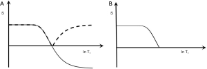
It is possible to extend the concept of multiplying two IR sequences together (as in the DIR sequence) to include addition, subtraction and fitting of two or more IR sequences as in the MASTIR (Multiplied, Added, Subtracted and/or fiTted IR) group of sequences. One example of this type of sequence is the Added IR (AIR) sequence. The T₁-filter for this sequence, in which phase-sensitive and magnitude reconstructed images with the same TI are added, is shown in Figure 25. It is a low pass T₁-filter.

Figure 25 T₁-filter for the Added IR (AIR) sequence. The phase sensitive (solid line) and magnitude (dashed line) reconstructed images are shown in (A) and are added and normalised in (B). This provides high signal for short T₁ tissues, and zero signal for longer T₁ tissues and fluids. It is a low pass filter.

Subtraction of a magnitude reconstructed image with an intermediate TI from a magnitude reconstructed image with a short TI is shown in Figure 26 (a Subtracted IR, or SIR sequence). It is a high pass, high transition band slope T₁-filter. In the central transition band there is up to twice the sensitivity to change in T₁ of the single IR sequences because both of these sequences contribute to it. In addition, the sign of the sequence weighting is positive.

Figure 26 T₁-filter for Subtracted IR (SIR) sequence with a linear T₁ scale. A magnitude reconstructed intermediate TI (green) image is subtracted from a magnitude reconstructed short TI image (red). The difference image (blue) shows that for T₁s in the range between the null points for the two TIs there is a very high positive slope (or sequence weighting) for the T₁-filter. The slope of the subtracted image in this range is greater than that of either of the original two IR images.

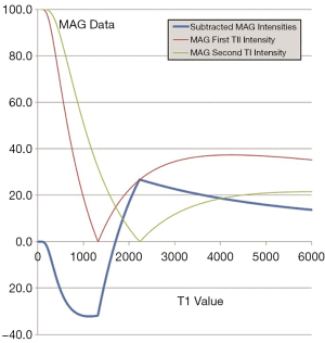
The sequence weighting for ρ_m and T₂ is synergistic with that for T₁ for concurrent increases in ρ_m, T₁ and T₂. For the intermediate TI sequence the T₁ sequence weighting is opposed to that of ρ_m and T₂ contrast. The opposed T₂ contrast can be reduced by using a short TE, or be made synergistic with the T₁ contrast using Echo Subtraction (ES).

The contrast synergy and high T₁ weighting of the SIR sequence are advantages compared with T₂-FLAIR sequences (where the T₁ contrast is opposed to that of ρ_m and T₂) for imaging of T₁s within the transition band. It is also an advantage compared with the heavily T₂-weighted SE sequence. CSF signal can be suppressed by multiplying the sequence by a long TI inversion filter (MSIR).

In summary the IR sequence T₁-filter has a high sloping regions. It includes negative signal values and options to null different tissues or fluids. It can be reconstructed in phase sensitive of magnitude form. Combinations of IR images can be used to null two or more tissues and to obtain high synergistic contrast.

The pulsed gradient spin echo (PGSE) sequence (TP-filter)

The D*-filter

The PGSE sequence is used to obtain D*-weighted images. The TP-filters are those of the basic SE sequence (Eq. [12]) with the inclusion of a fourth filter S_D* given by

The sequence weightings for C_ab and C_fr are:

where b is the diffusion sensitivity parameter and D* is the apparent diffusion coefficient. The PGSE sequence uses gradient pulses on either side of the 180° pulse to sensitize the sequence to diffusion. The b value for such a sequence is given by $\text{b}={\gamma }^2{G}^2{\delta }^2\left(\Delta -\frac{\delta }{3}\right)$ where γ is the gyromagnetic ratio, G is the gradient strength, δ is the duration of the sensitizing pulses and Δ is the separation in time between them. The symbols δ and Δ are used in this specific context with the PGSE sequence and do not represent chemical shift or change, as in earlier and later sections of this paper. When the gradient is applied almost continuously, b is approximately equal to $\frac{{\gamma }^2{G}^{2}T{E}^3}{12}$. In this situation (which is close to that often used clinically for maximum b value imaging) the diffusion sensitivity depends on G and TE. As a result, a single pulse sequence parameter TE affects both the T₂ and the D* weighting of the PGSE sequence. Diffusion weighted sequences usually include a reference “b = 0” (or in practice about 5-20 s/mm²) sequence with the same TR and TE as the principal sequence. These have a D*-filter which is essentially flat, and equal to 1 i.e., there is no filter effect for D*.

The D*-filter is shown in Figure 27. It is a negative exponential. The sequence weighting for C_ab is negative (middle row) and is opposed to that for TE. The first partial derivative of the filter which is the slope of the curve shown in red in the upper row goes through a negative maximum at bD* = 1 using a lnD* scale where the signal level is 37%. An increase in TE results in a shift of this curve to the left which is opposite to that for the SE T₂-filter. The sequence weighting for C_fr is shown in the lower row. There is no point of inflection. Signal from both the T₂ and D*^-filters decreases as TE is increased.

Figure 27 Plots of S_D* (the D*-filter using C_ab) (upper), $\frac{\partial {\text{S}}_{\text{D*}}}{\partial \text{In D*}}$ (the first partial derivative of this using C_ab) (middle) $\frac{1}{{\text{S}}_{\text{D*}}}$ and $\frac{\partial {\text{S}}_{\text{D*}}}{\partial \text{In D*}}$ (the D*-filter using C_fr) (lower) against lnD* for the PGSE sequence. S_D* is a negative exponential function. The partial derivative (middle) which is the D* sequence weighting shows a minimum at bD*=1 (vertical dotted line) for absolute contrast (C_ab). With fractional contrast (C_fr) (lower) there is no point of inflection for the sequence weighting.

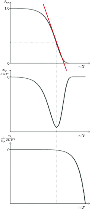
With a typical D*-weighted sequence (SE_TR/TE = 5,000/150 ms, b = 1,000 s/mm²) as used to examine gray matter of the brain with T₁=1,000 ms, T₂= 80 ms, and D*(gray) = 0.7x10^-3 mm²/s, the sequence weighting ratio is given by:

Although a sequence of this type is generally described as “diffusion weighted” using the qualitative approach, the dominant sequence weighting is actually from T₂ (46%) compared with -22% for diffusion. The same principles apply to the imaging of the liver tumors shown in Figure 5. The T₂ and D* weightings are opposed (i.e., they are of opposite sign). The term “shine through” is applied to the situation where a high signal is seen with a "diffusion weighted" image because of its concurrent heavy T₂-weighting and it may not be clear whether high signal seen in a lesion is associated with an increase or decrease in D*. Usually D* maps help by showing the magnitude and sign of the change in D*. However, with lesions with reduced T₂s, the overall image signal level may be low and diffusion weighting may result in little further reduction in this signal resulting in a noisy, spuriously low value of D* on the map.

Tumors

In the body, diffusion weighted images are frequently used to visualize tumors. The basic sequence is typically a STIR SE or a fat saturated SE sequence with an echo planar imaging (EPI) data collection. There is a fourth (diffusion) filter. If the tumor shows an increase in ρ_m, T₁, and T₂, but a decrease in D* i.e., $\frac{\Delta D^{*}}{D^{*}}$ negative then the diffusion contrast is positive and synergistic. It produces high overall contrast. A negative $\frac{\Delta D^{*}}{D^{*}}$ means that the tumor is more restricted than that in normal tissue. If $\frac{\Delta D^{*}}{D^{*}}$ is positive i.e., there is an increase in D*, the diffusion contrast is opposed to that produced from increases in ρ_m, T_1, and T₂ and the overall contrast may be low.

Subtraction of the D*-weighted sequence from the non-diffusion weighted sequence (b=0 s/mm²) can be used to reverse the D* contrast in this situation and make it synergistic with ρ_m and T₂ contrast for increases in all three of these tissue properties.

Anisotropy

In addition, basic diffusion contrast may be anisotropic and vary with orientation typically along, or across ordered fibers or cells. This is seen for example in white matter, skeletal and cardiac muscle, the kidney, tendons and ligaments. It is usually studied with gradients applied in a minimum of six directions to determine the diffusion tensor from which diffusion along and across major directions can be determined and expressed as fractional anisotropy. This is frequently reduced in disease. White matter has a normal D* that is low with the gradient transverse to the fiber direction. Disease in white matter producing an increase in D* in the direction transverse to the gradient may be indistinguishable from the normal higher D* seen in fibers which are parallel to the gradient direction.

Applications

High b value imaging is used to provide data for tractography using multi-directional gradients. Diffusion weighting is used with a low b value (e.g., b=50 s/mm²) to sensitize the sequence to perfusion where there is significantly larger motion of molecules of water than with diffusion. Low b values may also be used to suppress vascular signal in neurography and for assessment of perfusion as intravoxel incoherent motion.

Fat suppression is usually used with diffusion weighting (fat has a very low D* (e.g., 0.01 mm²/s) and would be high signal) and the signals from fluids are reduced because of their high D*. This results in low signal images which are usually tightly windowed. The fractional change in D* is often greater than those in T₁ or T₂ and if this is negative it often leads to high contrast.

In summary, the PGSE sequence adds a fourth (diffusion) filter to the SE sequence with sequence parameter b. TE controls both T₂-weighting and D*-weighting through b but the two sequence weightings are opposed. The T₂ sequence weighting is frequently greater than the diffusion sequence weighting. D* values are often decreased in important conditions such as acute cerebral infarction and many tumors which make the T₂ and D* image weightings synergistic and produce high signal. Anisotropy in white matter may lead to overlap between effects from normal and abnormal values of D*.

The SGE sequence (TP-filter)

Gradient echo sequences can be divided into: (I) SGE, (II) steady-state with free induction decay (FID) sampling, (III) steady-state with SE sampling, and (IV) balanced steady-state free precession (bSSFP) although other systems of classification are used (38-43). In this section the SGE sequence is considered and in the next section the bSSFP sequence is described.

The 180^o pulse in the SE sequence has a central role in reversing contrast effects in tissues with off-resonance frequencies different from water, such as those due to susceptibility differences and fat. With the gradient echo sequence, these effects are not reversed, and phase differences develop within, and between, voxels containing tissues with different resonant frequencies. The magnitude of the MR signal from a voxel is the complex sum of the signals from tissues within it. When these have different resonant frequencies and develop phase differences over time a reduction in signal magnitude results.

The SGE T₁, T₂, static field inhomogeneity (ΔB₀), susceptibility (χ), chemical shift (δ) and T₂*-filters are described next.

The T₁-filter

For the SGE sequences the signal for the T₁-filter is similar to that for the SE equation but with the addition of two flip angle (α) terms so that:

The signal is controlled by two sequence parameters TR and α. For a given TR the T₁-filters for flip angles of 90°, 70°, 50°, 30°, and 10° are shown in Figure 28A. As flip angle decreases from 90°, the signal and the slope of the T₁-filter decrease on the left, although signal may increase slightly on the right. The first partial derivative of the curve is shown in Figure 28B where it goes through a negative maximum. Maximum signal is obtained by putting $\frac{\partial S_{T_1}}{\partial \alpha }=0$ which gives the Ernst angle which is the value of α for maximum signal α_S, where

The flip angle for maximum contrast, α_c is obtained by putting $\frac{{\partial }^2{S}_{T_1}}{\partial \ln T_1\partial \alpha }=0$ for which

Figure 28 T₁-filter for SGE sequence. Plots of ${\text{S}}_{{\text{T}}_{\text{1}}}$ (A) and $\frac{\partial {\text{S}}_{{\text{T}}_{\text{1}}}}{\partial {\text{In T}}_1}$ (B) against lnT₁ for flip angles (α) of 90^o, 70^o, 50^o, 30^o and 10^o for the SGE sequence. As the flip angle decreases from 90^o (A), the slope of the curve decreases. At 10^o the curve is nearly flat over a wide range. (B) shows the sequence weighting which is negative and decreases as α decreases from 90° to 10°. The curve in (A) is identical to the T₁-filter for the SE sequence at α=90° but as α decreases the curve flattens. The value of T₁ for maximum sequence weighting shown in (B) increases as flip angle decreases.

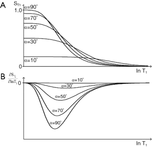
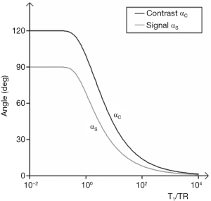
Plots of α_S and α_C are shown in Figure 29. The flip angle for maximum contrast is greater than that for maximum signal. For given values of TR and T₁, Figure 29 provides values of flip angles to maximize contrast or signal. These are much less than 90° for short TRs (cf. Figure 6). For long values of TR i.e., T₁/TR low, high flip angles (e.g., 80–90^o) result in high T₁ contrast, but for short values of TR (including those normally used with fast 3D sequences) T₁/TR is higher, and flip angles to maximize T₁ contrast are lower e.g., 5–30^o.

Figure 29 Plots of α_S (flip angle for maximum signal) and α_C (flip angle for maximum contrast) against T₁/TR for the SGE sequence. This curve gives values of T₁/TR to maximise signal and contrast. The flip angle for maximum contrast (α_C) is greater or equal to that for maximum signal (α_S). The curves reach a maximum on the left with low values of T₁/TR. At higher values of T₁/TR the flip angles for maximum signal and maximum contrast converge.

The T₂-filter

This generally follows that for the SE sequences except the relevant T₂ is T₂* (the apparent T₂) i.e., the T₂ modified by the effects of B₀ inhomogeneity and tissue susceptibility, as well as the presence of fat and contrast agents (see later).

Static field inhomogeneity (ΔB₀-filter)

Hitherto, all filters have shown signal magnitude along the Y axis in Cartesian (X,Y) coordinates but it is also possible to use radial (r,θ) coordinates and display both the signal and the phase of the signal in the form of TP-filters. The vector sum of signals from two tissues P and Q in a voxel is shown in Figure 30A, and the vector difference, or contrast between two voxels containing tissues P and Q respectively is shown in Figure 30B.

Figure 30 Vector addition (A) and subtraction (B) for two tissues P and Q. Vector addition of signal and phase for the tissues shows the resultant on the right as for intravoxel signal. Vector subtraction (B) shows the intervoxel contrast between P and Q in (B).

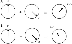
In the particular case where there is a Gaussian distribution of ΔB₀ within the voxel the phase dispersion results in a reduced T₂ * given by

Where ΔB₀ is the field inhomogeneity across the voxel.

Tissue susceptibility (χ-filter)

This can also be shown in radial form displaying signal magnitudes and the phase difference ∆θ between two tissues in separate voxels given by

Where γ is the gyromagnetic ratio, χ is the fractional susceptibility difference, B₀ is the magnetic field and TE is the echo time (Figure 31). The phase difference can be shown on a phase map. If there is a susceptibility difference between two or more tissues within a voxel then the signal magnitude and phase are obtained from the complex sum of all components. This usually results in reduced signal magnitude.

Figure 31 Phase TP-filter with linear phase (θ) on the Y axis and linear susceptibility on the X axis. The positive difference ∆χ from P and Q corresponds to a positive difference ∆θ for a given value of TE. As TE is increased the slope of the χ-filter is increased.

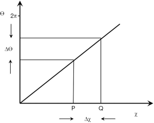
In addition, the χ of tissues containing ordered fibers may vary with their orientation to be zero such that

Where ϕ is the orientation of the fibers to the field.

There are also more sophisticated forms of modeling field effects which use a dipolar model of the field in a voxel and so produce more accurate maps of susceptibility.

The magnitude and phase signals can also be multiplied together in a form of Susceptibility Weighted Imaging (SWI) (44), see later section 18.

The chemical shift filter (δ-filter)

The phase difference between two signals ∆θ due to their chemical shift difference δ is given by:

Where γ is the gyromagnetic ratio, δ is the chemical shift difference B₀ is the static magnetic field, and TE is the echo time.

The filter is linear i.e., θ increases with δ for a given TE. The chemical shift difference δ between protons in water and those in the largest –CH₂ peak in triglycerides is about −3.3 ppm (i.e., the fat proton resonant frequency is 3.3 ppm lower than the water proton resonant frequency).

For a voxel containing a mixture of water and fat, the signal from the voxel is the vector sum of the complex signals from both tissues. When the phase difference is 0^o, 360^o, etc., signals simply add (i.e., in-phase, TE =4.4 ms at 1.5T for the water and –CH₂ peaks), but when the difference is 180^o the signals are opposed and the vector sum may be reduced or zero (out-of-phase, TE =2.2 ms at 1.5T).

The fat spectrum contains multiple peaks each with a different δ and these peaks show phase differences with a voxel containing fat alone the complex sum decreases with time as a result of phase interference effects.

Quantitation of ρ_m for fat is usually shown as the proton density fat fraction (PDFF) i.e., the ratio of ρ_m in fat to ρ_m for fat and water. This involves reducing or eliminating effects due to the differences in T₁ and T₂ between protons in water and the fat peaks as well as chemical shift effects utilizing multiple data points and prior knowledge of the fat spectrum.

The T₂*-filter

The observed T₂ may be reduced by inhomogeneity of the static field (ΔB₀), tissue susceptibility effects (including orientation), chemical shift effects (e.g., signals out of phase), and other effects. These can be represented by relaxation rates where

The rates are additive. They can be shown as a composite T₂*-filter, or as separate filters.

In summary, the SGE sequence has a low pass T₁-filter controlled by two sequence parameters TR and α. As α decreases from 90° the filter has less T₁-weighting than that of the corresponding filter in the SE sequence and flattens out. For a given TR, signal is maximized at the Ernst angle and T₁ contrast is maximized at higher values of α i.e., α_C. The SGE sequence has a T₂* filter which includes T₂ effects as well as those from static field inhomogeneity, tissue susceptibility, chemical shift, and contrast agents. The phase TP-filter shows intravoxel summation effects as well as intervoxel phase differences.

The bSSFP sequence (TP-filter)

The bSSFP sequence uses a gradient echo data acquisition and balances gradient areas along all three axes over each TR. It produces a signal which is the sum of FID and SE contributions. It is a GE sequence with SE properties. Although it does not have a 180^o pulse the off-resonance signals due to chemical shift and susceptibility are rephased at the time of data collection. Transverse magnetization is not spoiled (as it is with the SGE sequence) and contributes to the signal. To analyse the signal the T₁ and T₂ segments are combined as a single TP T₂/T₁. Tissues and fluids can be divided into four groups on this basis, namely watery hard tissues (T₂/T₁ ≈ 0.001) (usually very low signal), many watery soft tissues (T₂/T₁ ≈ 0.01), fat (T₂/T₁ ≈ 0.1), and fluids (T₂/T₁ ≈ 1) each approximately differing by an order of magnitude. Contrast between these groups can be high but varies with flip angle. Contrast within a group is usually lower. The sequence can produce high SNR per unit time and is used with magnetization preparations to provide T₁ and other contrast.

The T₂/T₁-filter for different flip angles is shown in Figure 32. The simplified filter (for TR << T1 or T2) (39) is:

Figure 32 T₂/T₁-filter for the bSSFP Sequence. Plot of S_T2/_T1 against lnT₂/T₁ for flip angles of 90°, 70°, 50°, 30°, and 10°. As the flip angle decreases from 90° to 10° the curve flattens.

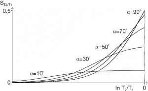
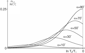
The first derivative which is the sequence weighting is shown in Figure 33. The flip angle for maximum signal (α_s) is given by:

Figure 33 First derivative of the T₂/T₁-filter or the sequence weighting for the bSSFP sequence. Plot of$\frac{\partial {\text{S}}_{{\text{T}}_2/{\text{T}}_{\text{1}}}}{\partial {\text{In T}}_2/{\text{T}}_1}$ against $\ln \frac{{\text{T}}_2}{{\text{T}}_1}$. For each flip angle α the sequence weighting is maximum at values of $\ln \frac{{\text{T}}_2}{{\text{T}}_1}$ given by cos ${\text{α}}_{\text{C}}\text{=}\frac{\text{1-}\frac{{\text{3T}}_{\text{2}}}{{\text{T}}_{\text{1}}}}{\text{1+}\frac{{\text{3T}}_{\text{2}}}{{\text{T}}_{\text{1}}}}$. As the flip angle decreases the value of T₂/T₁ for maximum sequence weighting decreases.

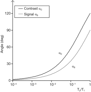
and that for maximum contrast α_c, by:

These are illustrated in Figure 34. For the common change in disease of soft tissues where T₁ and T₂ are both increased, the ratio T₂/T₁ may show relatively little change, and this may result in very little intrinsic contrast.

Figure 34 bSSFP sequence. Plot of flip angle for maximum contrast α_c, and maximum signal α_s against$\frac{{\text{T}}_{\text{2}}}{{\text{T}}_{\text{1}}}$. The flip angle for maximum contrast is greater than that for maximum signal.

In summary, the bSSFP sequence has a high pass T₂/T₁-filter. Contrast is high between bone and tendons, watery soft tissues, fat, and fluids but contrast within these groups e.g., soft tissues is low. Although T₁ and T₂ are both often increased in disease the ratio T₂/T₁ changes much less and sensitivity to disease is often low. The sequence is optimized for maximum signal. It is used as a localizer, or for data collection with magnetization preparation e.g., with an pulse inversion pulse.

The UTE sequence (TP-filter)

UTE sequences employ nominal TEs as short as 8 µs and are able to usefully detect signals from tissues with T₂s as short as 0.1 ms. Signal is typically acquired from a free induction decay using radial mapping of k-space and frequency encoding.

Related sequences employing ultrashort TEs include Zero TE (ZTE), Pointwise Encoding Time Reduction with radial Acquisition (PETRA) and SWeep Imaging with Fourier Transformation (SWIFT) behave similarly.

When the tissue T₂ is of the order of the duration, or less than the duration of the rf pulses used in the sequence, significant transverse relaxation occurs during the pulse. Long duration initial inversion pulses can be used to selectively invert and null long T₂ components, but leave short and ultrashort T₂ components uninverted. These can be subsequently detected with UTE data acquisitions.

Short and ultrashort T₂ components are frequently in a minority compared with long T₂ components and the signal from the latter may need to be suppressed in order to specifically visualize short T₂ components. This can be done by selectively inverting and nulling the long T₂ components, by ES i.e., subtraction of a longer TE image from a shorter TE one, and other methods.

The T₁-filter

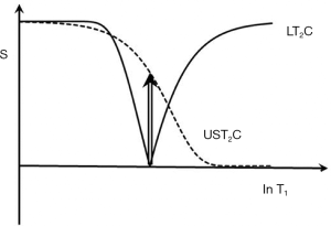
The long T₂ components experience an inversion pulse and their longitudinal magnetization can be nulled by choosing the correct TI. They follow a long TR (single) IR sequence T₁-filter pattern. Concurrently the ultrashort T₂ components are not inverted but are partially saturated and follow the T₁-filter of the SE sequence with TR equal to the TI of the IR-UTE sequence.

At the null time for the long T₂ components the ultrashort T₂ components have positive magnetization (Figure 35).

Figure 35 T₁-filter for the UTE-IR sequence. The long T₂ component (LT₂C) is inverted and nulled. The ultrashort T₂ component (UST₂C) is not inverted and shows positive signal at the time when the LT₂C is nulled.

The T₂*-filter

The T₂*-filter begins after the excitation pulse which creates transverse magnetization at TE₁ from short and ultrashort T₂ components as well as long T₂ components.

The ultrashort T₂ signals decay rapidly and are usually zero at the time of a second gradient echo acquisition at TE₂. ES with the longer TE image subtracted from the shorter TE image leads to a band pass filter selective for ultrashort and short T₂ components (Figure 36). If the long T₂ components have been successfully nulled by the use of an inversion pulse the overall signal at TE₂ is typically zero. The Double Echo Sliding IR-UTE [(DESIRE)-UTE] (45) sequence provides a range of TIs and the correct ones for nulling specific long T₂ components can be selected.

Figure 36 Echo subtraction. Two T₂-filters for a shorter TE₁ and a longer TE₂ are shown in (A) and the difference between them in (B) which is a band pass filter. It shows positive sequence weighting for shorter values of T₂ and negative sequence weighting for longer values T₂.

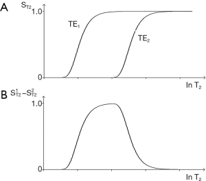
ES with a medium TE can also be used to reverse the contrast of the T₂*-filter in the medium T₂ range, and with a long TE to selectively reduce the signal from long T₂ fluids to zero.

Contrast agents—Gd-DTPA

In previous sections pulse sequences have been used as the starting point and tissue properties associated with them have been discussed, but it is also possible to start with a TP (such as the concentration of Gd-DTPA chelate within tissue, c and then consider pulse sequences. This is appropriate when the TP is relevant for many different pulse sequences.

Low molecular weight extracellular Gadolinium chelates (e.g., Gd-DTPA) are administered in bolus form for Dynamic Susceptibility Contrast (DSC) or at a slower rate as infusions for angiography and Dynamic Contrast Enhancement (DCE). There are also partially intracellular agents such as Gd-EOB-DTPA with a longer time course, and high molecular weight Gd polymers which are used as blood pool agents and persist in the circulation for longer times. The Gd chelates decrease T_1, T₂, and T₂* and change the signal of tissue water components more than that of fat components.

The effect of Gd-DTPA can be considered in two parts: (I) the effect of the contrast agent on the tissue properties T₁, T₂ and T₂*, and (II) the effect of these changes on image contrast using the relevant pulse sequence weightings. These are principally the T₁-filter with SE, IR and SGE sequences for conventional clinical contrast enhancement and DCE, and T₂*-filters with DSC usually with SGE and EPI sequences.

The effect of Gd-DTPA on T₁ and T₂

The effect of Gadolinium-DTPA on T₁ and T₂ is given by

and

Where r₁ and r₂ are the T₁ and T₂ relaxivities and c is the concentration of the contrast agent. The subscript b indicates baseline. The subscript c indicates T₁ or T₂ values after contrast administration. The fractional changes in T₁ and T₂ are given by:

and

These are shown in Figure 37.

Figure 37 Plot of change in T₁, ΔT₁ over baseline T_1b (ΔT1/T_1b) against concentration of Gd-DTPA, c (A). The curve asymptotically approaches -1 at high values of c. Plot of changes in ΔT₂ over baseline T_2b (ΔT₂/T_2b) against concentration of Gd-DTPA, c (B). The curve asymptotically approaches −1 as c increases.

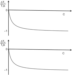
Image contrast produced by the reductions in T₁ and T₂

The contrast produced by the reductions in T₁ and T₂ are given by the fractional reductions in T_1b and T_2b multiplied by the sequence weighting of the chosen sequence. With T₁-weighted SE, SGE and intermediate TI IR sequences the T_1b reduction results in an increase in signal and contrast at lower values of c. Only at high values of c does the reduction in T_2b result in a negative contrast. A univariate T₁ filter can be used at low values of susceptibility effects are incorporated with T₂* and a univariate T₂ filter from SGE or EPI sequences can be used for the signal reduction.

Flow (TP-filter)

Flow affects are manifest in a variety of different ways. They usually involve blood and CSF as well as fluids in the bladder, joints, bursae, and cysts. Inflow of unsaturated fluid into a slice that has previously been excited and has not fully recovered may be manifest as a relative increase in signal as the fresh fluid displaces partially saturated fluid prior to the next data collection.

Signal may be lost when blood travels too quickly after the 90^o excitation and slice selection of a SE sequence to experience the subsequent localized 180^o pulse. Motion of a fluid at different velocities in the presence of a magnetic gradient may result in phase dispersion and loss of signal. Even echo rephasing may lead to increase in signal in a second echo.

For reasons of space we only consider phase changes due to flow with the PGSE sequence. This may be used to produce phase changes Δθ in flowing fluid where

γ is the gyromagnetic ratio, G is the strength of the gradient, δ is the duration of the gradient, Δ is the time between the gradient pulses (the definition of δ and Δ are the usual ones in this context but differ from those used earlier and later in this paper) and v is the velocity of blood. The phase shift is directly proportional to velocity. The filter is a TP-filter with velocity along the linear X axis and phase along the linear Y axis. The slope of the filter changes with G. The slope is low for low G values, and increased with higher values. Its maximum value is 2π radians, and the cycle is repeated at higher velocities (Figure 38).

Figure 38 Phase TP-filter for the PGSE sequence plotting θ against velocity v. The filter is linear over a 2π range. It has an increased slope at high gradient strength G (high G) (solid line) compared to low gradient strength (low G) (dashed line).

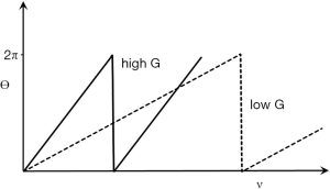
Phase TP-filters

The MR signal has a phase θ associated with it as well as the magnitude S. With conventional SE acquisitions the signal is rephased at the central time of detection so phase effects can be ignored. With UTE acquisitions there is little time to develop phase differences, but with SGE sequences there is time for them to develop and they may be significant.

The effects depend on whether they are:

• intravoxel where the phase and the signal is the vector sum of all the tissue components within the voxel at the time of data acquisitions (Figure 30A), or
• intervoxel where the contrast is the difference in phase and the difference in signal between two voxels or groups of voxels (Figure 30B).

The tissue properties of interest are ΔB₀ the (extrinsic) inhomogeneity of the static field B₀, χ or (intrinsic) tissue susceptibility, δ, velocity when encoded with a PGSE sequence and c, the concentration of paramagnetic contrast agent which produces susceptibility effects. ΔB₀ is property of the magnetic field, not of the tissue, but the static magnetic field induces temporary changes in the magnetic field within the tissue so that ΔB₀ effectively becomes a TP.

Tissue intrinsic susceptibility is a basic TP and includes effects from the presence of iron. It changes in disease [e.g., calcification (diamagnetic), and stages of hemorrhage [paramagnetic)].

The TP-filter equations for ΔB₀, χ, δ and v are respectively ∆θ=γ∆B₀, ∆θ=γχB₀, ∆θ=γδB₀, ∆θ=γδ∆Gv. The sequence weightings are γ, γχ, γ∆ and γδ∆G respectively. The phase contrast (absolute) ∆θ= sequence weighting x ΔTP. The phase TP-filters follows the same general principles as for signal magnitude as described previously, but are simpler. The changes scale with B₀ except for v.

The univariate model considers just one TP in a voxel and the phase of the signal follow from the sequence weighting and change in TP. Contrast is the difference in phase between two voxels.

The X axes of the TP-filters are those of the tissue properties and the scale is linear. The Y axes are phase, θ. This has a maximum value of 2π and then cycles from zero again. The θ scale is linear.

The multivariate model considers two or more tissue properties within the same voxel as well as contrast between two different voxels of this type.

Susceptibility weighted imaging (SWI) in the form described by Haacke et al. (44) multiplies the signal from a voxel by the high pass filtered phase of the signal (to eliminate effects from low frequency ΔB₀ variation).

Quantitative Susceptibility Mapping (QSM) uses ΔB₀ measurement and magnetic field modelling to produce a map of tissue χ alone.

PDFF imaging use multiple TE data correction for ΔB₀, fat spectral effects as well as T₁ and T₂ differences between water and fat to produce maps.

Magnetization preparation (TP-filters)

Pulse sequences have both preparation and acquisition components. In addition, there is often post-acquisition image processing as well as window width and levelling. Each of these have filters associated with them.

Magnetization preparation affecting the preparation stage of sequences do not include acquisitions, and so are used in conjunction with pulse sequences which do have these. Magnetization preparations may affect signal, contrast and weighting and can be regarded as TP-filters. Examples include fat saturation, selective water excitation, and MT.

There is overlap between pulse sequences and magnetization preparations. An inversion pulse may be regarded (I) as part of a pulse sequence and (II) as a form of magnetization preparation as with the MP-RAGE (Magnetization Preparation with Rapid Acquisition Gradient Echo) sequence. This sequence has contrast similarities to the long TR (single) IR group of sequences.

The effects of magnetization preparation on signal, contrast and weighting can be shown with TP-filters affecting the TP, the sequence weighting, or both.

Fat saturation and selective water excitation are examples of magnetization preparation affecting tissue properties. The TP filters for both are simple i.e., zero signal for fat along the X axis.

MT can be regarded as a form of magnetization preparation which affects the tissue properties ρ_m and T₁ which become the observed ρ_m, and the observed T₁ respectively (45,46). These effects can be shown on the X axes of the ${\text{S}}_{{\text{ρ}}_{\text{m}}}$ and ${\text{S}}_{{\text{T}}_{\text{1}}}$ filters respectively with many pulse sequences.

Using a classical model the fractional reduction observed in ρ_m is the same as the fractional reduction in observed T₁ (47). The two effects produce opposed contrast with SE sequences. The proton density sequence weighting is greater than that for T₁ making it the dominant effect.

MT does not affect fat or fluid so subtraction of an image with MT from one without MT results in both fat and fluid signal reduction or suppression.

In diseased tissue MT effects are often less than in normal tissue so that relative to normal tissue diseased tissue may behave as though it has an increase in ρ_m and an increase in T₁. These effects can be synergistic.

The MT ratio is (signal without MT minus signal with MT) over signal without MT. This depends on the changes in both ρ_m and T₁ and is a fractional change in contrast.

With the IR sequences MT pulses can be placed before the inversion pulse (in the TR period), after the inversion pulse (in the TI period) or in both places. The contrast effects of a reduction in ρ_m and T₁ are synergistic with STIR sequences and may be used to reduce the observed T₁ of muscle to that of fat so that both tissues are nulled.

MT subtraction (without MT minus with MT) reduces fat and fluid signals to zero and can be applied to IR sequences to obtain synergistic ρ_m, T₁ and T₂ contrast.

Other tissue properties: T₁ρ , the magic angle effect and temperature

These may also be modelled using TP filters. They include T₁ρ, the magic angle effect and tissue temperature.

T₁ρ

This is the longitudinal relaxation of magnetization during the application of the B₁ pulse at the resonant frequency. The decay is described by an exponential where

Where TSL is the time the spin lock is applied. This can be modelled in a similar way to the T₂ -filter of an SE equation.

Magic angle effect

This describes the fact that the T₂ of highly ordered collagen rich tissues such as tendons, ligaments, and menisci may vary with the orientation of the fibers to be zero (Θ) according to the equation

as a result of residual dipolar coupling.

Temperature

The temperature of tissue changes T₁ the resonant frequency and the coefficient D* to a first approximation the fractional increase in T₁ is proportional to absolute temperature, resonance frequency, and hence phase accumulated per unit time as well as the fractional change in diffusion.

Acquisition Filters (k-space filters)

Complex signal magnitude and phase data is acquired in MR imaging and is understood in terms of its location in 2D or 3D k-space. Signal in the central region of k-space is particularly associated with global image contrast and that in the peripheral region with spatial resolution.

If a high pass filter is applied in 2D to k-space so that the central regions are low or zero signal, image contrast is reduced and image edges and boundaries appear enhanced. If a low pass filter is applied, contrast appears increased and the image appears smoothed with less obvious boundaries.

The effects of re-ordering k-space on contrast are global, and are expressed throughout the image. They are incorporated in the signal scaling function, K. The filtering is of signals in k-space which have been affected by tissue properties; it is not direct filtering of tissue properties as with TP-filters.

With the fast SE sequence higher signals acquired at shorter TEs are often mapped to the center of k-space and lower signals acquired at longer TEs are mapped to the periphery of k-space, resulting in a loss of edge definition. The global contrast of the image is determined by the signals mapped to the center of k-space and the TE for these is described TE_eff. The KRISP sequence maps data acquired at, or around the null point to the center of k-space with data signal on either side of this point relatively decreased. This results in an edge enhancement effect on the images (48). This can also be done for T₂ using K-space Weighted Image Contrast (49).

Image processing filters (S-filters)

Image processing can be performed in many different ways. The Fourier transformation of an image can be used to filter it in the frequency domain or the signal of an image can be convolved with a filter in the spatial domain using a kernel to calculate the value of each voxel as a function of the signal in voxels adjacent to it. This approach can be used to smooth images to decrease their spatial resolution and increase their contrast. It can also be used for edge enhancement. The X axis of the filter is signal intensity, not a TP so that this is an S-filter not a TP-filter. Its effects are manifest through the image scaling function, K.

The combination of two or more images (S, TP and spatial filters)

Two or more images can be combined in different ways. This includes subtraction (e.g., post intravenous contrast administration minus pre-contrast administration) and using two or more images with an exponential model relating them to calculate T₁, T₂ or D*.

Each image may be signal processed, as described previously (S-filter), before combination, and after combination. Subtraction of a post-enhancement image from a pre-enhancement one produces a difference image whose contrast is modulated by c and can be described by a TP-filter.

Other subtractions may be between two MR images that differ in one or more sequence parameters (e.g., SIR). These are also TP-filters even if they are processed after acquisition, not acquired during the preparation stage of the sequence. MTRs are another example.

SWI, as described by Haacke et al. (44) where a signal magnitude image is multiplied by a high pass filtered phase image acquired at the same data collection is a TP-filter.

When two images acquired at different times (e.g., pre- and post-contrast enhancement) it is usually necessary to align the images before subtracting one from the other. This can be done with a pure spatial filter that translates and rotates the image using rigid body registration without changing the signal of the images. More complex deformable registration can be used where there is a change in the spatial properties of the second image over time in order to align them. These are spatial filters affecting the location of images in space, not their signals.

Saturation bands are preparation spatial filters with the detected signal level zero.

Images from different modalities e.g., MR and PET may be fused. This is also a spatial filter not a TP-filter.

Both TP and spatial filters can operate in the preparation and the post acquisition image processing stages.

The combination of two or more images may be described by S-filters, TP-filters and spatial filters of different types. TP-filters describing changes in signal and contrast can be used both in the preparation and post-acquisition stages of sequences or images.

Window width and level (S-filter)

Changing the window width and level of an image display changes the original image signal S to a new signal display signal, S_D. The effect is that of linear high pass filter of S with the addition of a magnification factor so that typically S_D = mS + c over the signal range of the transition band of the filter. This results in an increase in the display contrast by the factor m (Figure 39) which is manifest in the image scaling function, K. It is not a TP-filter, but looks similar to the SIR T1-filter shown in Figure 26.

Figure 39 Effects of window width and level. (A) is a plot of display signal (S_D) against signal (S) showing a linear relationship for two tissues P and Q. If the S_D difference for P and Q (S_DQ–S_DP) is expanded to occupy the whole display range by narrowing the window width as in (B), absolute contrast on the display is increased. The effect is that of a high pass S-filter (thick lines) in (B) with amplification of the signal and contrast in the transition band between P and Q.

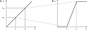
With fractional contrast, low signal level contrast is amplified more than higher signal contrast leading to a relative increase.

The physiological optical response to signal as perceived brightness is logarithmic (the Weber-Fechner law), so fractional contrast may correspond more closely to the human perception of contrast rather than absolute contrast. Given a free option to choose window level and contrast, observers may opt more for the equivalent of fractional contrast when viewing lower signal levels.

In Figure 39, the contrast of relatively low signals is increased to correspond to the signal levels on the display. This re-scales absolute contrast towards fractional contrast. This is relevant for low signal sequences such as T₂-FLAIR, fat saturated FSE in the musculoskeletal system and diffusion weighted sequences. As a result, for the T₂-FLAIR sequence the optimization for T₂ weighting may not be at TE=T₂ as for C_ab, but may be given by TE/T₂ as for C_fr. With C_fr scaling, increasing TE increases contrast up until the point where the image becomes signal to noise limited. This may help explain the observer preference for very long TEs with the T₂-FLAIR sequence.

Signal to noise ratio (SNR) and contrast to noise ratio (CNR)

So far we have mainly considered signal and contrast but these are always accompanied by noise, and both the signal level at which contrast is produced and the background noise are of central importance. The SNR is an important index of machine performance and sets an upper limit on CNR. The SNR is also important in the low signal situation where normalization of the signal and weighting ratios become invalid.

CNR is related to the detectability of differences since these are seen against background of noise. It is common to compare absolute contrast to noise on the grounds that the noise and signal are scaled together so that this represents a form of normalization and improves the validity of comparisons. C_fr is scaled relative to tissue signals.

The image noise level reflects voxel size, time of acquisition, bandwidth, coil performance and other factors and is usually regarded as uniformly distributed throughout the image although this may not be true of images obtained with partially parallel techniques.

Phase mages are used for δ, χ and v. These are single property images and values can be read off directly. In that sense they are univariate and 100% weighted for the relevant TP. They are limited by noise and phase to noise ratio, as well as phase contrast to noise ratio.

TP maps and synthetic images

Tissue maps and synthetic images are univariate and display values of a single TP. They have been used in clinical MRI since 1983. They form the basis for primary diagnosis with PDFF imaging, detection of fibrosis in myocardium by measurement of T₁, and determination of iron in the heart in thalassemia using T₂*. Such maps are supplement to multi TP images in diffusion imaging where D* maps may help determine increases and decreases in D* when these are confounded by the concurrent T₂-weighting. Single TP maps have the substantial advantage of unambiguous interpretation of their weighting and overall simplicity in directly supplying the information of interest i.e., differences in TP and changes in the TP in disease.

The problems include:

• Often the calculation involves a ratio of 0/0 which is undefined in parts of the image and may give very high/very low values reducing confidence in the validity of the rest of the image.
• The maps may show potentially troublesome partial volume effects from high TP tissues or fluids such as CSF which are not present on the multi tissue property images (e.g., CSF on T₂ maps compared with T₂-FLAIR images, and D* maps of fluids compared with PGSE images).
• The sequence acquisition for TP values may not be appropriate for high or low TP values e.g., very short or very long T₂ values leading to no calculation, or significant errors.
• The model for signal analysis e.g., single component may be inappropriate.
• The data acquisition necessary for accurate values may be too time consuming in clinical practice.
• Artefacts may be manifest in unusual ways on maps compared with source images and may not be recognized.
• There are wide variations in the published normal values for tissue properties such as T₁ and T₂.

However, the situation has improved recently with the advent of fingerprinting (50) and other techniques e.g., ShMOLLI (51) which provide more accurate TP values in reasonable scan times. This data is important in its own right, and is also valuable for calculating weighting in health and disease in individual patients, as well as in wider populations.

Other types of weighting

We have concentrated on the main types of weighting seen clinically but there are 30–40 different types of weighting described in the English language imaging literature. These (I) often follow directly from the Bloch equations (as for ρ_m, T₁ and T₂ above), or (II) are linked to them with a specific relationship (as with contrast agents). There is also a third class with less well defined changes where the sequence weighting or change in tissue properties, or both are not fully characterized for which weighting is described in qualitative terms.

In this paper about ten tissue properties have been considered (of 20 or more), as well as about ten sequences or magnetization preparations (of many more). These choices reflect current clinical usage.

Summary

The conventional approach to weighting is qualitative and describes a sequence or an image by the TP (e.g., T₁, T₂) most responsible for the contrast of interest using terms such as T₁-weighted and T₂-weighted. The TP-filters approach treats pulse sequences as filters of tissue properties (e.g., T₁, T₂) and shows them in graphical form including the voxel signal S, the contrast (difference in signal, ΔS between two tissues) and the sequence weighting (slope of the filter) for each TP. The approach may be used in univariate form (one TP-filter at a time) or in multivariate form with two or more TP-filters considered together. TP-filters are summarized in Table 6.

Table 6 TP-filters in graphical form
Full table

For the univariate model a filter has:

• Along the X axis:
• Tissue properties such as ρ_m, T₁, T₂, D*
• The X axis can be linear with differences in values ΔTP, or
• Logarithmic with differences in value ΔlnTP = ΔTP/TP. The X axis can be rescaled to log₁₀ x using log₁₀ x = log x = lnx/ln10
• Along the Y axis:
• For signal:
• Signal. This is voxel signal normalized to a maximum value of 1, or 100%.
• Contrast. This is the difference in signal between two voxels and can be intrinsic for the same tissue (e.g., normal and abnormal) or extrinsic (two different tissues).
• It can be absolute C_ab = ΔS the difference in signal with a linear Y axis, or fractional C_fr = ΔS/S with a logarithmic Y axis.
• For phase:
• This is voxel phase normalized to 100% (=2π radians)
• Contrast is difference in phase between two voxels
• The scale is linear
• The filter equation is of the form S = ρ_m (1−TR/T₁). ${\text{e}}^{-{\text{TE/T}}_2}$ (for the SE sequence). The variables are the tissue properties ρ_m, T₁ and T₂. The times TR and TE are fixed.
• Sequence parameters are used to specify the filter e.g., TR, and TE for the SE sequence; TR, TI, TE for the IR sequence; TR, TE, and b for the PGSE sequence.
• The first partial derivative of theTP-filter with respect to TP, or lnTP i.e., ΔSTP/ΔTP or ΔSTP/Δ(lnTP) is the slope of the filter, and this is the sequence weighting for that TP. The sequence parameters describing the first partial derivative of the filter are the same as those describing the filter i.e., TR, TE, TI etc.
• The second partial derivative of the filter can be used to determine points of inflection of the first derivative and so maximize contrast. For example, using C_ab and a lnT₁ X scale for the SE sequence this occurs at TR = T₁ and TE = T₂ for the T₁ and T₂-filters of the SE sequence. The values are TR=2T₁ and TE=2T₂ for a linear T₁ and T₂ X scale.
• Image contrast C_ab or C_fr is the product of sequence weighting (slope of the filter curve) and the change in TP, either ΔTP (linear) or ΔlnTP = ΔTP/TP (logarithmic).
• The image weighting (i.e., the proportion of the contrast C_ab or C_fr originating from each TP is ±100% using the univariate model for each TP-filter (e.g., T₁ or T₂) since all the contrast arises from a single TP.
• C_ab and C_fr can be used to measure differences in contrast between two tissues, and in conjunction with the sequence weighting can be used to calculate values of ΔTP or ΔTP/TP i.e., the TP change responsible for the contrast.
• Positive or negative signs are assigned to each of S, Contrast, change in TP, sequence weighting and image weighting as well as the X and Y axes.
• The univariate model provides a mathematical formalism for converting conventional qualitative weighting (which is univariate) to quantitative weighting.
• The multivariate model considers two or more TP-filters, such as the three TP- filters of the SE sequence, using the TP-filters for each TP. The sequence parameters controlling the sequence are those for each of the constituent filters.
• The multivariate model provides sequence weighting ratios $\text{s}{W}_{SEQ}^{\text{r}}({\rho }_m:T_1:T_2:\mathrm{..})$ which give the percentage contribution of each TP to the overall sequence weighting.
• The model also provides image weighting ratios $i{W}_{SEQ}^{\text{r}}({\rho }_m:T_1:T_2:\mathrm{..})$ which give the percentage contribution of each TP to the overall image contrast.
• The contrast can be used with the $\text{s}{W}_{SEQ}^{\text{r}}$ to calculate ΔTP or ΔTP/TP.
• There is no equivalent to multivariate weighting using conventional qualitative weighting.
• Four groups of filters are described, namely:
• TP-filters (signal and phase)
• Acquisition filters (k-space)
• Signal filters e.g., (S-filters) e.g., post acquisition image processing filters, and window width and level filters. These are signal filters not TP- filters.
• Spatial filters. These can be used for example to change image position, but not voxel signal.
  TP-filters are classified by the quantity along their X axes. They are also usually specified using descriptive terms e.g., linear, exponential, low pass, high pass, band pass, notch. The transition bands between stop and pass bands are usually the regions of most clinical relevance.
• TP-filters are applicable in both the preparation stage of sequences and in post acquisition image processing.

Conclusions

It is possible to define TP-filters (linear exponential, low pass, high pass, notch, double notch, linear, band pass, etc.) which directly relate the signal and contrast of images to tissue properties with different sequences. TP-filters provide a range of functions of the type originally envisaged by Godfrey Hounsfield over 40 years ago for the T₁ and the IR sequence. Other antecedents include Kurtz and Dwyer (52), Buxton et al. (42) and Pelc (34) who used partial derivatives to optimize image contrast, as well as Elster who described an index system to assess comparative parameter weighting (53), and an earlier paper on the mathematics underlying weighting (54). These papers generally addressed mathematical formalism rather than clinical applications or the underlying concepts. The TP-filter approach resolves ambiguities and uncertainties associated with the use of the conventional univariate qualitative approach to imaging. The TP-filter formulation provides a formalism for understanding signal contrast and weighting comparable to that which k-space provides for signal localization and global contrast.

The TP-filter model can be understood and used at five levels:

• Weighting can be regarded essentially as a label and used freely for purposes such as scheduling where image interpretation is not required.
• It is also possible to use the conventional qualitative weighting terminology, but use it in a way that recognizes and avoids obvious contradictions or ambiguities.
• The third level is using TP-filters either singly or in combination in graphical form. The patterns of signal, contrast and weighting with different sequences can be understood using with TP-filters without the need for precise TP values. Useful reference points are where TR=T₁, TI=T₁, TE=T₂, bD*=1 etc.) to place the filters along the X axis. Graphs of the filters are shown in Table 6.
• The fourth level is using TP-filters in mathematical form. Filter equations, first and second partial derivatives, sequence parameter values to maximize contrast and normalized first partial derivatives are shown in Table 7. This provides an overview as well as specific information e.g., normalized partial derivatives to calculate sequence and image weighting ratios.
• The fifth level is as a computer Application (App) with normal TP data at the relevant field strength, and pulse sequence data so that filters can be displayed. Changes in tissue properties can be calculated from them and displayed when required. In addition, the inclusion of relevant abnormal TP values may help with recognition and characterization of pathological changes.

Table 7 TP-filters in mathematical form
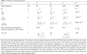
Full table

Acknowledgments

Funding: The authors acknowledge grant support from NIH (1R01 NS092650).

Footnote

Conflicts of Interest: All authors have completed the ICMJE uniform disclosure form (available at http://dx.doi.org/10.21037/qims.2020.04.07). JD serves as an unpaid editorial board member of Quantitative Imaging in Medicine and Surgery. The other authors have no conflicts of interest to declare.

Open Access Statement: This is an Open Access article distributed in accordance with the Creative Commons Attribution-NonCommercial-NoDerivs 4.0 International License (CC BY-NC-ND 4.0), which permits the non-commercial replication and distribution of the article with the strict proviso that no changes or edits are made and the original work is properly cited (including links to both the formal publication through the relevant DOI and the license). See: https://creativecommons.org/licenses/by-nc-nd/4.0/.

References

1. Bates S, Beckmann L, Thomas A, Waltham R. Godfrey Hounsfield: intuitive genius of CT. London, UK: British Institute of Radiology, 2012.
2. Wells PNT. Sir Godfrey Newbold Hounsfield KT CBE 28 August 1919-12 August 2004. Biogr Mems Fell R Roc 2005;51:221-35. [Crossref]
3. Young IR. Hounsfield, Sir Godfrey Newbold (1919-2004), Oxford Dictionary of National Biography. doi 2009. [Crossref]
4. Isherwood I. Sir Godfrey Hounsfield. Radiology 2005;234:975-6. [Crossref]
5. Hounsfield GN. Computed medical imaging. In: J Lindsen. editor. Nobel lectures Physiology or Medicine. Singapore: Singapore World Scientific Publishing Co, 1992:1971-80.
6. Twieg DB. The K-trajectory formulation of the NMR imaging process with applications in analysis and synthesis of imaging methods. Med Phys 1983;10:610-21. [Crossref] [PubMed]
7. Ljunggren S. A simple graphical representation of Fourier-based imaging methods. J Mag Res 1983;54:338-48.
8. Bryant D, Bailes DR. NMR imaging. Contemporary Physics 1984;25:441-75. [Crossref] [PubMed]
9. Bailes DR, Young IR, Thomas DJ, Straughan K, Bydder GM, Steiner RE. NMR imaging of the brain using spin echo sequences. Clin Radiol 1982;33:395-414. [Crossref] [PubMed]
10. Brady TJ, Rosen BR, Pykett IL, McGuire MH, Mankin HJ, Rosenthal DI. NMR imaging of leg tumors. Radiology 1983;149:181-7. [Crossref] [PubMed]
11. McGinnis BD, Brady TJ, New PF, Buonanno FS, Pykett IL, DeLaPaz RL, Kistler JP, Taveras JM. Nuclear magnetic resonance (NMR) imaging of tumors in the posterior fossa. J Comput Assist Tomogr 1983;7:575-84. [Crossref] [PubMed]
12. Glossary of NMR Terms. Magn Reson Med 1984;1:414-33. [Crossref] [PubMed]
13. Anonymous. Instructions to contributors. J Comp Assist Tomogr 1984;8(1): (no page number).
14. Anonymous . Publication information for authors. J Magn Reson Imaging 1991;1:109-11.
15. American College of Radiology. Glossary of NMR Terms. 2nd ed. Reston, VA: American College of Radiology, 1986.
16. Axel L. Revised glossary of MR terms. Radiology 1987;162:874. [Crossref] [PubMed]
17. Mitchell DG, Vinitski S, Rifkin MD, Burk DL Jr. Sampling bandwidth and fat suppression: effects on long TR/TE MR imaging of the abdomen and pelvis at 1.5 T. AJR Am J Roentgenol 1989;153:419-25. [Crossref] [PubMed]
18. Aoki S, Okada Y, Nishimura K, Barkovitch AJ, Kjos B, Brasch RC, Norman D. Normal deposition of brain iron in childhood and adolescence: MR imaging at 1.5 T. Radiology 1989;172:381-5. [Crossref] [PubMed]
19. Davis PC, Hoffman JC Jr, Ball TI, Wyly JB, Braun IR, Fry SM, Drvaric DM. Spinal abnormalities in pediatric patients: MR imaging findings compared with clinical, myelographic, and surgical findings. Radiology 1988;166:679-85. [Crossref] [PubMed]
20. Hesselink JR, Dowd CF, Healy ME, Hajek P, Baker LL, Luerssen TG. MR imaging of brain contusions: a comparative study with CT. AJR Am J Roentgenol 1988;150:1133-42. [Crossref] [PubMed]
21. American College of Radiology. Glossary of MR Terms. 3rd ed. Reston, VA: American College of Radiology, 1991.
22. American College of Radiology. Glossary of MR Terms. 4th ed. Reston, VA: American College of Radiology, 1995.
23. American College of Radiology. Glossary of MRI Terms. 5th ed. Reston, VA: American College of Radiology, 2005.
24. Rinck PA, Muller RN, de Francisco PA. Glossary of MRI Terms. European Magnetic Resonance Forum. Updated June 9 2007. Accessed October 16, 2007. Available online: http://www.emrf.org
25. Wehrli FW. Fast-scan Magnetic Resonance principles and applications. New York, NY: Raven Press, 1991:145-48.
26. Nishimura DG. Principles of Magnetic Resonance Imaging. Palo Alto: Stanford University, 2010.
27. Buxton RB. Introduction to functional magnetic resonance imaging, 2nd edition. Cambridge: Cambridge University Press, 2009.
28. Parker DL, Tsuruda JS, Goodrich KC, Alexander AL, Buswell HR. Contrast-enhanced magnetic resonance angiography of cerebral arteries. A review. Invest Radiol 1998;33:560-72. [Crossref] [PubMed]
29. Bottomley PA, Foster TH, Argersinger RE, Pfeifer LM. A review of normal tissue hydrogen NMR relaxation times and relaxation mechanisms from 1-100 MHz: dependence on tissue type, NMR frequency, temperature, species, excision, and age. Med Phys 1984;11:425-48. [Crossref] [PubMed]
30. Rooney WD, Johnson G, Li X, Cohen ER, Kim SG, Ugurbil K, Springer CS Jr. Magnetic field and tissue dependencies of human brain longitudinal 1H2O relaxation in vivo. Magn Reson Med 2007;57:308-18. [Crossref] [PubMed]
31. Reichert IL, Robson MD, Gatehouse PD, He T, Chappell KE, Holmes J, Girgis S, Bydder GM. Magnetic resonance imaging of cortical bone with ultrashort TE pulse sequences. Magn Reson Imaging 2005;23:611-8. [Crossref] [PubMed]
32. Robson MD, Gatehouse PD, Bydder M, Bydder GM. Magnetic resonance: an introduction to ultrashort TE (UTE) imaging. J Comput Assist Tomogr 2003;27:825-46. [Crossref] [PubMed]
33. Panda A, Obmann VC, Lo WC, Margevicius S, Jiang Y, Schluchter M, Patel IJ, Nakamoto D, Badve C, Griswold MA, Jaeger I, Ponsky LE, Gulani V. MR fingerprinting and ADC mapping for characterization of lesions in the transition zone of the prostate gland. Radiology 2019;292:685-94. [Crossref] [PubMed]
34. Pelc NJ. Optimization of flip angle for T1 dependent contrast in MRI. Magn Reson Med 1993;29:695-99. [Crossref] [PubMed]
35. Hendrick RE. Contrast and image noise. In: Stark DD, Bradley WG. editors. Magnetic Resonance Imaging, 3rd ed. St Louis: Mosby,1999: 43-67.
36. Bydder GM, Young IR. MR. Imaging: clinical use of the inversion recovery sequence. J Comput Assist Tomogr 1985;9:659-75. [Crossref] [PubMed]
37. Redpath TW, Smith FW. Technical note: use of a double inversion recovery pulse sequence to image selectively gray or white brain matter. Br J Radiol 1994;67:1258-63. [Crossref] [PubMed]
38. Elster AD. Gradient echo MR imaging: techniques and acronyms. Radiology 1993;186:1-8. [Crossref] [PubMed]
39. Scheffler K, Lehnhardt S. Principles and applications of balanced SSFP techniques. Eur Radiol 2003;13:2409-18. [Crossref] [PubMed]
40. Bernstein MA, King KF, Zhou XJ. Handbook of MRI Pulse Sequences. Amsterdam: Elsevier, 2004:596.
41. McRobbie DW, Moore EA, Graves MJ, Prince MR. MRI from picture to proton. 2nd edition. Cambridge: Cambridge University Press, 2007:236-57.
42. Buxton RB, Edelman RR, Rosen BR, Wismer GL, Brady TJ. Contrast in rapid MR imaging: T1- and T2-weighted imaging. J Comput Assist Tomogr 1987;11:7-16. [Crossref] [PubMed]
43. Neelavalli J, Haacke EM. A simplified formula for T(1) contrast optimization for short-TR steady-state incoherent (spoiled) gradient echo sequences. Magn Reson Imaging 2007;25:1397-401. [Crossref] [PubMed]
44. Haacke EM, Xu Y, Cheng YC, Reichenbach JR. Susceptibility weighted imaging (SWI). Magn Reson Med 2004;52:612-8. [Crossref] [PubMed]
45. Ma YJ, Searleman AC, Jang H, Wong J, Chang EY, Corey-Bloom J, Bydder GM, Du J. Whole-brain myelin imaging using 3D Double-Echo Sliding Inversion REcovery Ultrashort Echo Time (DESIRE UTE) MRI. Radiology 2020;294:362-74. [Crossref] [PubMed]
46. Henkelman RM, Stanisz GJ, Graham SJ. Magnetization transfer in MRI: a review. NMR Biomed 2001;14:57-64. [Crossref] [PubMed]
47. Hajnal JV, Baudouin CJ, Oatridge A, Young IR, Bydder GM. Design and implementation of magnetization transfer pulse sequences for clinical use. J Comput Assist Tomogr 1992;16:7-18. [Crossref] [PubMed]
48. Oatridge A, Curati WL, Herlihy AH, Hajnal JV, Virji N, Puri BK, Bydder GM. Evaluation of a FLAIR sequence designed to reduce CSF and blood flow artifacts by use of k-space reordered by inversion time at each slice position (KRISP) in high grade gliomas of the brain. J Comput Assist Tomogr 2001;25:251-6. [Crossref] [PubMed]
49. Song HK, Dougherty L. Dynamic MRI with projection reconstruction and KWIC processing for simultaneous high spatial and temporal resolution. Magn Reson Med 2004;52:815-24. [Crossref] [PubMed]
50. Ma D, Gulani V, Seiberlich N, Liu K, Sunshine JL, Duerk JL, Griswold MA. Magnetic resonance fingerprinting. Nature 2013;495:187-92. [Crossref] [PubMed]
51. Piechnik SK, Ferreira VM, Dall'Armellina E, Cochlin LE, Greiser A, Neubauer S, Robson MD. Shortened Modified Look-Locker Inversion recovery (ShMOLLI) for clinical myocardial T1-mapping at 1.5 and 3 T within a 9 heartbeat breathhold. J Cardiovasc Magn Reson 2010;12:69. [Crossref] [PubMed]
52. Kurtz D, Dwyer A. Isosignal contours and signal gradients as an aid to choosing MR imaging techniques. J Comput Assist Tomogr 1984;8:819-28. [Crossref] [PubMed]
53. Elster AD. An index system for comparative parameter weighting in MR imaging. J Comput Assist Tomogr 1988;12:130-34. [Crossref] [PubMed]
54. Yokoo T, Bae WC, Hamilton G, Karimi A, Borgstede JP, Bowen BC, Sirlin CB, Chung CB, Crues JV, Bradley WG, Bydder GM. A quantitative approach to sequence and image weighting. J Comput Assist Tomogr 2010;34:317-31. [Crossref] [PubMed]