ADAPTIVE-NET: deep computed tomography reconstruction network with analytical domain transformation knowledge
Introduction
In medical computed tomography (CT) imaging applications, image reconstruction plays a critical role in visualization and interpretation. Conventionally, the most widely used CT image reconstruction methods are all based on analytical algorithms like the filtered-back-projection (FBP) CT reconstruction algorithm (1,2) for parallel-beam and fan-beam imaging geometry, and the Feldkamp Davis Kress (FDK) CT reconstruction algorithm (3) for cone-beam imaging geometry. Although the analytical CT image reconstruction algorithms are fast, it is difficult to produce high-quality CT images with them when the radiation dose is reduced. Therefore, over the past two decades, optimization-based iterative CT image reconstruction algorithms, which include imaging models, prior information, and proper regularization (4-10) have been adopted as the dominant solutions for CT image denoising and artifact removal. In contrast to the analytical FBP and FDK algorithms, the iterative algorithms usually need an assumed CT image to compute the forward projections, compare the original projection data, and update the assumed CT image based upon the difference between the calculated and the actual projection data. However, optimization-based iterative CT image reconstruction algorithms usually require longer computation times.
Recently, the deep learning technique, which has already become popular in computer science (11), has attracted research interest from the medical imaging fields. In CT image reconstruction applications, some pioneering studies (12-20) have demonstrated that the deep learning technique, especially the deep convolutional neural network (CNN), can be used to reduce the noise and artifacts on FBP and FDK reconstructed CT images. Technically, the CNN-based methods implemented in prior studies have attempted to reduce CT image noise and artifacts via an image-domain post-processing procedure. For example, Chen et al. (13) proposed a residual encoder-decoder CNN (RED-CNN) to reduce image noise in low dose CT (LDCT). In this study, the network input was the LDCT images reconstructed with an FBP algorithm, and the network output was the CT images with a standard dose level. Zhang et al. developed a CNN-based method to reduce streaking artifacts in sparse view CT imaging (18). Similarly, the network input was the FBP-algorithm-reconstructed sparse view CT images containing severe streaking artifacts, and the network output was the CT image reconstructed from a full view scan. One advantage of using CNN over iterative CT image reconstruction algorithms is that it takes less time to reconstruct CT images. However, it should be noted that a CNN network always needs to be trained in advance, and this training time is not counted in the CT image reconstruction time.
Rather than starting the CNN-based CT image reconstructions from noise or artifacts degraded CT images, one recent study (21) demonstrated that CT images could be reconstructed directly from the acquired Radon projections (also known as the sinogram) by a properly designed end-to-end supervised CNN. Zhu et al. reframed the CNN network as an “automated transform by manifold approximation” (AUTOMAP). In this new paradigm, CNN learns the complicated mathematical CT image reconstruction procedure (21,22), including both the domain transformation and data filtration. However, the use of fully connected (FC) layers makes the AUTOMAP network difficult to implement, especially when the CT image to be reconstructed has a clinically relevant dimension. For example, to reconstruct a typical CT image 512×512 in dimension, the FC layers in AUTOMAP may occupy up to hundreds of gigabytes of GPU memory, which is a challenge to handle for a workstation equipped with only a limited number of GPUs. To solve this issue, we suggest replacing the FC layer-based domain transformation which is used in the AUTOMAP network with the conventional analytical back-projection-based domain transformation (23,24). Since such analytical back-projection operations can be easily implemented with a finite computation resource, a CT image can, therefore, be reconstructed from an end-to-end supervised CNN network on a single GPU with moderate memory capacity. In this work, we have coined the term “ADAPTIVE-NET” to refer to the newly developed analytical domain-back-projection-driven CT image reconstruction network.
The following methods section presents details of the ADAPTIVE-NET, including the network architecture, loss function, and error backpropagation mechanism. In the experiment section, the training data generation, network training, and quantitative evaluations are discussed. In the results section, details of the comparison results are presented for the eight methods. We discuss the relevant implications of our work and the major conclusions in the discussion and conclusion sections, respectively.
Methods
CT imaging model
Assuming the CT system has a parallel-beam imaging f (x, y) geometry, the projection of an arbitrary 2D object on the detector plane at a certain view-angle θ can be written as follows:
|
| [1] |
In Eq. [1], p(r, θ)denotes the measured Radon projection, δ(xcosθ+ysinθ−r)specifies an x-ray beam passing through the object, r is the distance from the origin (x =0, y =0) to the beam, and θ is the angle between the +y-axis to the ray penetrating the object. For the parallel-beam imaging geometry, the projections are usually acquired with a 180-degree tube-detector rotation interval, namely, 0≤ θ ≤π. With the linear algebra language, Eq. [1] can be rewritten as the following:
|
| [2] |
where matrix A represents the forward Radon projection model. To reconstruct the object f(x, y) from the acquired projection data p(r, θ), the FBP algorithm is usually used. In this algorithm, the original projection data p(r, θ) needs to be filtered first with certain types of filtering kernels. Afterward, one needs to put each projection value back into the object space along the Radon integration direction one view after another. By doing so, a reconstructed image of the object f(x, y), denoted as ffbp(x, y), in the CT image domain can be obtained. This procedure can be expressed by the following equation:
|
| [3] |
where F denotes the project data filtering procedure. Similarly, Eq. [3] can be denoted as
|
| [4] |
Here, AT represents the adjoint of the forward projection operation A. Thus, AT denotes the back-projection operation. Essentially, the back-projection operation AT plays the role of domain transformation from the projection domain to the CT image domain.
User-developed FBP operator in TensorFlow
We here propose to make the FBP procedure an individual network layer, rather than a group of CNN layers as has been previously implemented by Würfl et al. (23,24). However, there is no such build-in component readily available in the TensorFlow platform, and thus we developed it independently. In TensorFlow, this component is called an operator. By design, this self-developed operator accepts a group of system parameters and performs filtration and back-projection during network training. The system parameters include the source-to-detector distance, the source-to-iso-center distance, the detector element size, the total view numbers, and others. The standard ramp filter was used, and the filtered data was back-projected into the CT image domain in a voxel-driven manner. The corresponding gradient back-propagation operator was also developed. To be compatible with the TensorFlow platform, all calculations were implemented by CUDA (25).
ADAPTIVE-NET
Using our own self-developed operators, we had the opportunity to build a new end-to-end CT image reconstruction network by jointly accessing the sinogram domain and the CT image domain. As illustrated in Figure 1, three individual units are cascaded one after the other to work simultaneously during CT image reconstructions. In particular, the forefront projection domain unit (PDU) is used to extract features on the sinogram. It has three convolutional layers, and the kernel size is 1×3. The middle unit is responsible for domain transformation from the sinogram domain to the CT image domain. The third unit (IDU) is designed to perform feature extractions in the CT image domain. In this study, we made use of the RED-CNN as the third unit. Compared with the RED-CNN, one potential advantage of ADAPTIVE-NET is that the original information stored in the sinogram can be accessed directly, ensuring the use of raw data information during CT image reconstructions. Under this condition, the ADAPTIVE-NET becomes an extended version of the RED-CNN. In ADAPTIVE-NET, both the sinogram domain processing and the CT image domain processing are performed at the same time. To validate the performance of the ADAPTIVE-NET, we would use it for LDCT image reconstructions.

Loss functions
In this study, two types of loss functions were used. One was the mean square error (MSE) loss defined as follows:
|
| [5] |
Here, denotes the Frobenius norm, Nx and Ny represent the number of CT image pixels along with the horizontal and vertical directions, respectively. The reference CT image is denoted as I, and the CT image reconstructed from CNN is denoted as ICNN.
The other loss used is defined as a weighted summation of MSE loss and VGG loss (26) as expressed in the following equation:
|
| [6] |
where λ is a hyperparameter to balance the MSE loss and VGG loss. In particular, the VGG loss is useful in characterizing the similarity between two images. Often, the pre-trained VGG16 CNN network is chosen to measure the similarity between two images. By definition, the VGG loss LVGG is expressed as the following:
|
| [7] |
where VGGn is the squared feature difference at the n-th pooling layer of the pre-trained VGG16 network, and is the number of channels of feature maps at the n-th pooling layer. In this study, we empirically set n from 1 to 5 for the natural denoising of LDCT images.
Error back-propagation in ADAPTIVE-NET
Assuming the network loss function is L, the gradients of network variables in the IDU (assuming it is in the j-th layer of ADAPTIVE-NET) can be immediately expressed as follows:
|
| [8] |
where l denotes the output of a certain network layer. All the calculations are routine and based on the chain rule. The gradients of network variables in the PDU (assuming it is in the i-th layer of ADAPTIVE-NET and positioned in front of the DTU) can be expressed as follows:
|
| [9] |
As discussed previously, the self-developed operators responsible for analytical CT image reconstructions by default are designed to be constants. In the forward network propagations, the operation O=ATF is utilized to perform CT image reconstructions. Conversely, in the backward network propagations, it is the following:
|
| [10] |
Specifically, the network gradients calculated automatically in the IDU stage have to be scaled by FTA times in order to estimate the variable gradients in the PDU stage during all the ADAPTIVE-NET gradient back-propagations.
Training dataset
The Mayo LDCT challenge dataset was used to generate the network training data. First, a linear transformation was applied to convert the clinical CT image [Hounsfield unit (HU)] to the linear attenuation coefficient µ (unit of 1/mm) as follows:
|
| [11] |
where the factor 0.02/mm corresponds to the reference X-ray linear attenuation coefficient of water around 60 keV. This is a close approximation to most of the mean X-ray tube energy in routine clinical CT scans. Second, fan-beam CT imaging geometry was simulated. In particular, the source-to-detector distance was 1,270.00 mm, and the source-to-rotation center was 870.00 mm. There are 1,000 detector elements, each with a dimension of 0.80 mm. We assumed that all CT images have the same pixel dimension of 0.625 mm × 0.625 mm. Forward projections (i.e., Radon projections) were collected from 900 views with a 0.4-degree angular interval. Both the quantum Poisson noise and the Gaussian electronic noise were added in simulations. Poisson noise was added to each simulated projection with the entrance mean photon number of 5×10⁴ per ray. In addition, zero-mean Gaussian noise with a noise-equivalent-quanta of 10 photons per ray was also added into the projection data to mimic the electronic noise. In total, 5,413 data pairs were collected: 4,887 pairs were used to train the network, and the remaining 526 pairs were used to validate the network. All the above numerical operations were performed in Python.
Comparison schemes
In this study, images were reconstructed from the seven following algorithms for comparison: the LDCT image reconstructed by FBP (denoted as LDCT), the iterative reconstruction algorithm with total variation (TV) regularizer processed image (denoted as TV), the CT image generated from the RED-CNN method with MSE loss (denoted as RedCNN-MSE), the CT image generated from the RED-CNN method with combined MSE loss and VGG loss when λ=1,000 (denoted as RedCNN-VGG-1000*MSE), the CT image generated from the ADAPTIVE-NET with MSE loss (denoted as ADAPTIVE-MSE), the CT image generated from the ADAPTIVE-NET with combined MSE loss and VGG loss when λ=5,000 (denoted as RedCNN-VGG-5000*MSE), and CT image generated from the ADAPTIVE-NET with combined MSE loss and VGG loss when λ=1,000 (denoted as RedCNN-VGG-1000*MSE).
Algorithm implementation
For the TV-based iteration algorithm, the weight of the TV regularizer was set to 0.02, and the number of iterations was selected to achieve the lowest NMSE for each individual image.
During the training of the RED-CNN network and ADAPTIVE-NET, the network automatically updated the weights and biases for all channels, and gradually learned the optimal parameters to minimize the loss function L. Specifically, the Adam algorithm was used with a starting learning rate of 0.00001, which exponentially decayed by a factor of 0.98 after every 1,000 steps. The mini-batch had a size of 1, and batch-shuffling was turned on to increase the randomness of the training data. The network was trained for 100 epochs on Tensorflow deep learning framework using a single NVIDIA GeForce GTX 1080Ti GPU. Once being trained, the ADAPTIVE-NET took about 0.3 seconds to reconstruct 1 CT image of 512×512 from a sinogram of 1,000×900.
Quantitative evaluation metrics
The performances of the different CT image reconstruction methods were compared via several different quantitative evaluation metrics: normalized root mean square error (NRMSE), the structural similarity index metric (SSIM), peak signal-to-noise ratio (PSNR), and the noise power spectrum (NPS).
The NRMSE is defined as the following:
|
| [12] |
where x denotes the reconstructed image and x0 denotes the corresponding reference image.
|
| [13] |
where µ denotes the mean value of the image, σ2 denotes the variance of the image, and σa,b denotes the covariance of two images. In our calculations, C1=(0.01×R)2, and C2=(0.03×R)2, where R is the value range of image x. The images used to calculate SSIMs were 512×512 in size. Moreover, the 2D NPS was calculated from 200 noise-only samples with the following equation :
|
| [14] |
In Eq. [14], ∆u and ∆v are the image pixel size along axis u and v, respectively, and Nu and Nv are the total number of pixels along axis u and v, respectively. The averaged noise-only image was estimated from 200 samples as follows:
|
| [15] |
Results
Parameter selections
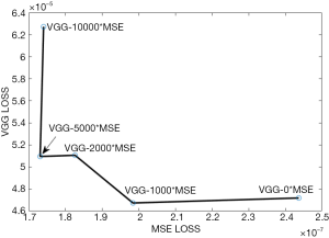
As shown in Eq. [6], the value of hyperparameter λ needs to be pre-determined in order to generate the most optimal LDCT imaging results. For this purpose, we empirically selected five different λ values: 10,000, 5,000, 2,000, 1,000, and 0.
For each value, the network was trained independently. Once the network converged, both the MSE loss and the VGG loss were calculated and drawn together to obtain the corresponding L-curve, as shown in Figure 2. According to the obtained L-curve, we selected two λ values: 5,000 and 1,000. Results were compared between them.
Imaging results
Figure 3 illustrates the lung imaging results with different reconstruction methods, and Figure 4 shows the zoomed-in region of interest (ROI) images. Visually, images reconstructed from the TV algorithm had strong plastic textures, and the spatial resolution was also poor. Both the RedCNN-MSE and ADAPTIVE-MSE methods could be used to improve the image quality, and the proposed ADAPTIVE-MSE method outperformed the RedCNN-MSE in recovering the fine anatomical lung structures, as circled in Figure 4. Overall, the images generated from the combined MSE loss and VGG loss had better image quality than that with only MSE loss. For the lung imaging study, the results obtained from different λ values looked quite similar.
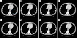
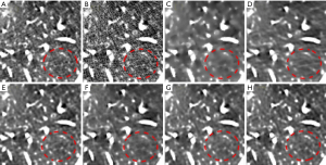
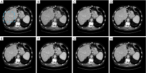
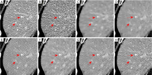
Figure 5 illustrates the results of one abdominal image, and Figure 6 shows the zoomed-in ROI images around the liver region. Again, images reconstructed from the RedCNN-MSE and ADAPTIVE-MSE methods had better spatial resolution than those reconstructed from the TV algorithm. With the MSE loss, the newly developed ADAPTIVE method generated better image spatial resolution than RED-CNN. Finally, images generated from combined MSE loss and VGG loss had better quality than those with only MSE loss. However, the zoomed-in image in Figure 6E contains strong checkboard artifacts, while they become less significant if processed by the proposed ADAPTIVE-NET with VGG loss. Additionally, the result in Figure 6H demonstrates that λ=1,000 can better reserve the natural-looking features of the reconstructed LDCT.
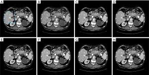
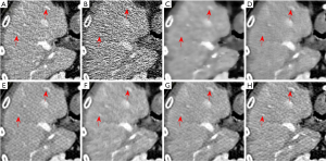
Images in Figures 7 and 8 illustrate results from another abdominal image. As can be seen, the RedCNN-MSE and ADAPTIVE-MSE methods generate images with better spatial resolution than those reconstructed from the TV algorithm. When only using the MSE loss, the newly developed ADAPTIVE method was able to generate LDCT images with slightly better image spatial resolution than the RED-CNN. When combining the MSE loss and VGG loss together, the reconstructed LDCT images looked more natural. However, the RED-CNN method contained strong checkboard artifacts. On the other hand, the checkboard artifacts were less significant when processed by the proposed ADAPTIVE-NET with VGG loss. Additionally, the result in Figure 8H demonstrates that λ=1,000 generates more natural-looking CT images than λ=5,000.
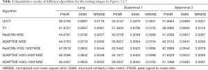
Moreover, quantitative comparisons were also conducted for a single test image and all 526 pairs of test images. For different body parts, taking the PSNR as an example, the Red-CNN-MSE and ADAPTIVE-MSE algorithms gained higher value than the TV method. More importantly, the joint use of VGG loss could further improve the PSNR values of both the RED-CNN and ADAPTIVE-NET method to very similar levels, as seen in Table 1. Our experiments found that even the ADAPTIVE-VGG-1000*MSE method was able to generate the most natural-looking LDCT images; however, the quantitative indices derived from it are slightly (<5%) lower than the highest achievable values. These results indicate that the loss functions may impact the quantifications, and this has been found in a previous study as well (27).
Full table
Across different body parts, the same quantitative measurements were performed and averaged, with the results being summarized in Table 2. Overall, the joint use of VGG loss could indeed enhance the network performance and thus generate better LDCT images. Again, all the CNN methods with and without VGG loss had similar quantitative outcomes (difference less than 5%).

Full table
Noise power spectrum (NPS) analyses
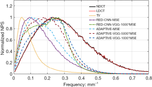
The measured noise power spectra for each CT image reconstruction method are presented in Figure 9. These 1D curves were generated by radially averaging the 2D NPS maps, which were generated from 200 independent noise-only samples. The ADAPTIVE-VGG-1000*MSE method had the best performance in terms of preserving the NPS shape and generating the most natural-looking LDCT images on par with the standard FBP-reconstructed NDCT images. The NPS curves obtained from RED-CNN-VGG-1000*MSE and ADAPTIVE-VGG-5000* MSE methods had very similar shapes but tended to have stronger low-frequency correlations and less significant high-frequency correlations. Compared with the RED-CNN-MSE algorithm, the new ADAPTIVE-MSE method exhibited more high-frequency correlations. The TV based-method showed the strongest shift towards the low-frequency range, indicating dramatic image blurring. Because the LDCT images reconstructed from the ADAPTIVE-VGG-1000*MSE method had the closest visual performance to the NDCT images, we chose it as the candidate reconstruction algorithm for our LDCT imaging application.
Discussion
In this paper, we propose a new end-to-end supervised CT image reconstruction network by incorporating the analytical domain transformation knowledge. With this newly developed ADAPTIVE-NET, high-quality LDCT images having clinically relevant dimensions of 512×512 and are able to be reconstructed directly from the full sinogram on a single GPU.
Essentially, the idea of integrating CNN and analytical domain transformation knowledge together has already been proposed in other recent literature. For example, Würfl et al. demonstrated that it is possible to map the FBP and FDK type CT image reconstruction algorithms into a CNN (23,24). In these studies, domain transformation was precisely implemented via analytical back-projection, which was embedded in the entire network as a specific layer with fixed constant weights. Since these networks are designed faithfully with the purpose of mapping the FBP and FDK type CT image reconstruction algorithms, it is likely difficult to use them for solving most typical problems related to CT reconstruction tasks, like LDCT reconstruction. To overcome this issue, we thought of modifying the network architecture to make it more general for end-to-end network-based CT image reconstructions. From this, we proposed the new ADAPTIVE-NET architecture.
In order to train the ADAPTIVE-NET, a full-size sinogram and NDCT image are needed. Unlike the RED-CNN network, the new network is not able to work with patched data, a patched sonogram, or a patched NDCT image. This requirement may potentially increase the number of full-size NDCT images used for network training. However, the benefit of using full-size sinogram data and NDCT image data in preserving the natural textures of the reconstructed LDCT images is also apparent. To compare, in this study, we also trained the RED-CNN with a full-size CT image, rather than using a patched CT image. With the same number of training data, results demonstrated that the ADAPTIVE-NET was able to outperform the RED-CNN. We thought this was because the ADAPTIVE-NET has the ability to simultaneously access the information stored in the original projection data and the reconstructed CT image. Because of the combination of projection information and CT information, results indicated that the proposed ADAPTIVE-NET would be more efficient than the RED-CNN in generating high-quality CT images, especially for LDCT imaging applications. Notice that the RED-CNN purely works in the CT image domain, and has been implemented as the image domain unit of the proposed ADAPTIVE-NET (Figure 1).
The value of parameter λ defined in Eq. [6] needs to be carefully selected to balance the contribution of MSE loss and VGG loss. Moreover, the value of λ may also depend on the imaging task. Different values may lead to different final results, such as image quality, noise correlation property, and so on. In this study, λ=1,000 was considered as one of the best selections for ADAPTIVE-NET when trained with joint MSE loss and VGG loss. This is because, in this case, the measured image quantification indices, such as SSIM, PSNR, and NRMSE, can reach a fairly high level. Additionally, the obtained NPS curve from ADAPTIVE-NET under this condition also has the closest shape to the NPS curve obtained from FBP-reconstructed CT images. Due to the high similarities, the reconstructed LDCT images with λ=1,000 from ADAPTIVE-NET have a more natural-looking appearance than the conventional NDCT images.
As seen in Figure 1, the proposed ADAPTIVE-NET in this study contains three cascaded units, with each one being responsible for a specific task. The forefront projection domain unit is used to extract features on the sonogram, the domain transformation unit is used to transform the sinogram into the CT image domain, and the image domain unit is used to extract features on CT images. Although we validated the ADAPTIVE-NET for LDCT imaging by exactly following the three-unit network structure, the illustrated three-unit structure in Figure 1 could be varied. For example, the first PDU might be abridged. In this condition, the ADAPTIVE-NET immediately becomes the RED-CNN network. If we further modify the network structure of the IDU, as has been done previously (28), then the ADAPTIVE-NET can be used as a back-projection-filtration CNN network. In contrast, the IDU might also be removed. In this case, the ADAPTIVE-NET will acquire a very similar network structure as those proposed by Würfl et al. (23,24). Specifically, it would become a CNN-based FBP or FDK CT image reconstruction algorithm. Therefore, the ADAPTIVE-NET is truly adaptable to certain applications.
In addition to being applicable for LDCT imaging, as demonstrated in this study, the new ADAPTIVE-NET can also be used in other CT image reconstruction tasks, such as the limited-view CT image reconstruction, the limited-angle CT image reconstruction, and in other conditions. This network is not only practicable in CT imaging but also has the potential for positron emission tomography (PET) and single-photon emission computed tomography (SPECT) image reconstruction applications. In brief, the ADAPTIVE-NET is truly adaptable to both the network architecture and imaging applications.
Future research will focus on performing comprehensive comparisons with the state-of-art CT imaging networks (29-32) for varied scenarios. In addition, we would also like to investigate the other potential imaging applications of ADAPTIVE-NET, as briefly discussed above.
Conclusions
We developed a novel end-to-end supervised CT image reconstruction network which incorporates an analytical back-projection domain transform layer to directly reconstruct CT images of clinically relevant dimensions from a full sinogram on a single GPU of moderate memory size. Due to the direct access and use of the projection information in ADAPTIVE-NET, the quality of the reconstructed LDCT image can be improved. In addition, the use of VGG loss is beneficial in generating more natural-looking LDCT images.
Acknowledgments
The authors would like to thank Dr. Cynthia McCollough (the Mayo Clinic, USA) for providing clinical CT data. We would like to acknowledge Dr. Tianye Niu from Zhejiang University for inspiring discussions.
Funding: This project was supported by the National Natural Science Foundation of China (Grant No. 11804356 and No. 81871441), the Guangdong Basic and Applied Basic Research Foundation (Grant No. 2019A1515011262), and Chinese Academy of Sciences Key Laboratory of Health Informatics (Grant No. 2011DP173015). The funding sponsors have no role in the collection, analysis, or interpretation of the data or in the decision to submit the manuscript for publication.
Footnote
Conflicts of Interest: The authors have no conflicts of interest to declare.
References
- Kak AC, Slaney M. Principles of Computerized Tomographic Imaging. IEEE Inc, 1988.
- Hsieh J. Computed tomography: principles, design, artifacts, and recent advances. SPIE Bellingham, WA, 2009.
- Feldkamp L, Davis L, Kress J. Practical cone-beam algorithm. JOSA A 1984;1:612-9. [Crossref]
- Stayman JW, Fessler JA. Regularization for uniform spatial resolution properties in penalized-likelihood image reconstruction. IEEE Trans Med Imaging 2000;19:601-15. [Crossref] [PubMed]
- Elbakri IA, Fessler JA. Statistical image reconstruction for polyenergetic X-ray computed tomography. Medical Imaging. IEEE Trans Med Imaging 2002;21:89-99. [Crossref] [PubMed]
- Sidky EY, Kao CM, Pan X. Accurate image reconstruction from few-views and limited-angle data in divergent-beam CT. J Xray Sci Technol 2006;14:119-39.
- Chen GH, Tang J, Leng S. Prior image constrained compressed sensing (PICCS): A method to accurately reconstruct dynamic CT images from highly undersampled projection data sets. Med Phys 2008;35:660-3. [Crossref] [PubMed]
- Yu H, Wang G. Compressed sensing based interior tomography. Phys Med Biol 2009;54:2791. [Crossref] [PubMed]
- Hara AK, Paden RG, Silva AC, Kujak JL, Lawder HJ, Pavlicek W. Iterative reconstruction technique for reducing body radiation dose at CT: feasibility study. AJR Am J Roentgenol 2009;193:764-71. [Crossref] [PubMed]
- Yu Z, Thibault JB, Bouman CA, Sauer KD, Hsieh J. Fast model-based x-ray CT reconstruction using spatially nonhomogeneous ICD optimization. IEEE Transactions on Image Processing 2011;20:161-75. [Crossref] [PubMed]
- LeCun Y, Bengio Y, Hinton G. Deep learning. Nature 2015;521:436. [Crossref] [PubMed]
- Kyong Hwan Jin. McCann MT, Froustey E, Unser M. Deep convolutional neural network for inverse problems in imaging. IEEE Transactions on Image Processing 2017;26:4509-22. [Crossref] [PubMed]
- Chen H, Zhang Y, Kalra MK, Lin F, Chen Y, Liao P, Zhou J, Wang G. Low-dose CT with a residual encoder-decoder convolutional neural network. IEEE Trans Med Imaging 2017;36:2524-35. [Crossref] [PubMed]
- Wang G, Ye JC, Mueller K, Fessler JA. Image reconstruction is a new frontier of machine learning. IEEE Trans Med Imaging 2018;37:1289-96. [Crossref] [PubMed]
- Han Y, Ye JC. Framing U-Net via deep convolutional framelets: Application to sparse-view CT. IEEE Trans Med Imaging 2018;37:1418-29. [Crossref] [PubMed]
- Kang E, Chang W, Yoo J, Ye JC. Deep convolutional framelet denosing for low-dose CT via wavelet residual network. IEEE Trans Med Imaging 2018;37:1358-69. [Crossref] [PubMed]
- Yang Q, Yan P, Zhang Y, Yu H, Shi Y, Mou X, Kalra MK, Zhang Y, Sun L, Wang G. Low-dose CT image denoising using a generative adversarial network with Wasserstein distance and perceptual loss. IEEE Trans Med Imaging 2018;37:1348-57. [Crossref] [PubMed]
- Zhang Z, Liang X, Dong X, Xie Y, Cao G. A sparse-view CT reconstruction method based on combination of densenet and deconvolution. IEEE Trans Med Imaging 2018;37:1407-17. [Crossref] [PubMed]
- Yang W, Zhang H, Yang J, Wu J, Yin X, Chen Y, Shu H, Luo L, Coatrieux G, Gui Z. Improving low-dose CT image using residual convolutional network. IEEE Access 2017;5:24698-705.
- Liu J, Ma J, Zhang Y, Chen Y, Yang J, Shu H, Luo L, Coatrieux G, Yang W, Feng Q. Discriminative feature representation to improve projection data inconsistency for low dose CT imaging. IEEE Trans Med Imaging 2017;36:2499-509. [Crossref] [PubMed]
- Zhu B, Liu JZ, Cauley SF, Rosen BR, Rosen MS. Image reconstruction by domain-transform manifold learning. Nature 2018;555:487. [Crossref] [PubMed]
- Cybenko G. Approximations by superpositions of a sigmoidal function. Math Control Signals Systems 1989;2:183-92. [Crossref]
- Würfl T, Ghesu FC, Christlein V, Maier A. Deep learning computed tomography. International Conference on Medical Image Computing and Computer-Assisted Intervention. Springer, 2016:432-40.
- Würfl T, Hoffmann M, Christlein V, Breininger K, Huang Y, Unberath M, Maier AK. Deep learning computed tomography: Learning projection-domain weights from image domain in limited angle problems. IEEE Trans Med Imaging 2018;37:1454-63. [Crossref] [PubMed]
- Gao H. Fast parallel algorithms for the x‐ray transform and its adjoint. Med Phys 2012;39:7110-20. [Crossref] [PubMed]
- Justin J, Alahi A, Li F. Perceptual Losses for Real-Time Style Transfer and Super-Resolution. Computer Vision-ECCV 2016. Springer International Publishing, 2016.
- Kim B, Han M, Shim H, Baek J. A performance comparison of convolutional neural network‐based image denoising methods: The effect of loss functions on low‐dose CT images. Med Phys 2019;46:3906-23. [Crossref] [PubMed]
- Ge Y, Zhang Q, Hu Z, Chen J, Shi W, Zheng H, Liang D. Deconvolution-based backproject-Filter (BPF) computed tomography image reconstruction method using deep learning technique. Med Phy 2018. arXiv preprint arXiv:1807.01833
- Wu D, Kim K, El Fakhri G, Li Q. Iterative low-dose CT reconstruction with priors trained by artificial neural network. IEEE Trans Med Imaging 2017;36:2479-86. [Crossref] [PubMed]
- He J, Wang Y, Yang Y, Bian Z, Zeng D, Sun J, Xu Z, Ma J. LDCT-Net: Low-dose CT image reconstruction strategy driven by a deep dual network. Medical Imaging 2018 Physics of Medical Imaging 2018;10573:105733.
- Li Y, Li K, Zhang C, Montoya J, Chen GH. Learning to reconstruct computed tomography (CT) images directly from sinogram data under a variety of data acquisition conditions. IEEE Trans Med Imaging 2019;38:2469-81. [Crossref] [PubMed]
- Yin X, Zhao Q, Liu J, Yang W, Yang J, Quan G, Chen Y, Shu H, Luo L, Coatrieux JL. Domain Progressive 3D Residual Convolution Network to Improve Low-Dose CT Imaging. IEEE Trans Med Imaging 2019;38:2903-13. [Crossref] [PubMed]

