

Topics on quantitative liver magnetic resonance imaging
Introduction
Liver magnetic resonance imaging (MRI) is subject to continuous technical innovations through advances in hardware, sequence and contrast agent development. When compared to its main competitor CT, MRI has the advantage of without ionizing radiation exposure, better tissue contrast, administration of contrast agent is not obligatory and if administered, contrast agent is of much smaller volume and hepatocyte-specific contrast agents are available. Liver MRI typically includes T1 weighted imaging (T1W), T2 weighted imaging (T2W), diffusion weighted imaging (DWI) and apparent diffusion coefficients (ADC) mapping, and contrast agent enhanced imaging. More recent developed quantification techniques of practical values include quantification of liver fat and iron, MR elastography, and dynamic contrast-enhanced (DCE) imaging.
Constraints associated with liver MRI include high cost, long acquisition time, greater need for patient collaboration and individual patient limitations such as claustrophobia and presence of pacemakers/metal implants, etc. Liver imaging is particularly susceptible to various physiological movements, particularly respiratory motion and cardiac motion for the left liver. A number of strategies, including external trigger techniques, have been developed for reducing or eliminating liver motion influences. Methods to speed up data acquisition are also introduced to overcome the constrains for liver imaging. As the availability of high field and ultra-high-field whole body MR system increase, the B1 inhomogeneity, and high specific absorption rate (SAR) and safety concerns also increased. There is a need for better coil design, acceleration techniques, and sequences to address these issues.
In order to utilize the abilities of liver MR to its full extent and perform high-quality efficient exams, it is mandatory to use the best imaging protocol, to minimize artifacts and to select the most adequate type of contrast agent. In this article, we review the routine clinical MR techniques applied currently and some latest developments of liver imaging techniques to help radiologists and technologists to better understand how to choose and optimize liver MRI protocols that can be used in clinical practice.
Liver fat signal suppression
Fat suppression is commonly used in MRI to suppress the signal from adipose tissue and can have abnormalities other than the adipose tissue enhanced, which will otherwise be bright signal due to their long T2. Fat signal suppression is achieved through two principles: (I) the difference in the resonance frequency between lipid and water protons, which is also called chemical shift (1). (II) the difference in T1 between lipid and water protons. The application of fat suppression techniques depends on the amount of adipose tissue to be suppressed in MR signal as well as the field-of-view (FOV) location relative to the field center (2,3).
Short TI inversion recovery (STIR) sequence uses an inversion pulse and time delay (TI) according to T1 of fat protons (2). In order to suppress signal from adipose tissue by nulling its longitudinal magnetization, so that fat will not contribute to signals in the subsequent image signal acquisition, an inversion-recovery pulse with specific timing is applied. The longitudinal magnetization of fat protons recovers faster than of water. Consequently, after a time delay [TI, usually 165 and 220 ms on 1.5T (T) and 3T MR, respectively] selected for the more rapidly-recovering fat signal reaches zero, a 90° pulse flips the magnetization into the transverse plane so that the fat transverse magnetization is zero. While the water protons still had a negative z component and pertain transverse magnetization signal. Image contrast between tissues depends on the tissue T1 values as well as the selected TI. However, the dependency of relatively long inversion recovery time sometimes causes conflicts with the respiratory trigger and causes images sensitive to motion. In addition, the intuitive SNR of STIR image relatively lower than the other fat suppression techniques described below. Hence this method is currently only limited applied in liver imaging.
Another family of fat-suppression pulse sequences are based on chemical shift effect or its hybrid technique with STIR. The difference in electronic shielding of the protons in fat molecules and water molecules results in different precession frequencies of fat and water (chemical shift effect). The fat peak is approximated 3.5 ppm away from water peak in MR spectroscopy (4), with the main fat peak’s resonance frequency 447 Hz lower than that of water at 3T, 223 Hz lower at 1.5T and 149 Hz lower at 1T (3). It is more effective for the frequency selective fat suppression methods at 3T compared with a weaker magnetic field because the two peaks are separated wider with higher magnetic field strength, other than potentially overlapped in a weaker magnetic field and cause heterogeneous fat suppression. However, frequency selective fat suppression methods are less suitable for a large field of view, off-center imaging and anatomic regions with challenging geometric features because of the higher B0 heterogeneity, neither for patients with metallic implants due to the strong susceptibility effect.
The STIR method can be modified with a combination of chemical selective or spectral pre-saturation attenuated inversion-recovery pre-pulses [spectral pre-saturation with inversion-recovery (SPIR)] (1,5). A spectral fat suppression RF preparation pulse is applied to rotate only the fat magnetization with an angle of 180°. The fat magnetization is then flipped in the z-direction, and starts the longitudinal relaxation. After a time TI, selected to null fat signal, the 90° excitation pulse is applied. As fat has no longitudinal magnetization at this point, the excitation pulse produces no fat transverse magnetization, therefore, the fat signal is suppressed. SPIR is mostly applied in T2W. Particularly because of its short pulses, it is used with multi-shot imaging methods, such as periodically rotated overlapping parallel lines with enhanced reconstruction (PROPELLER) and radial acquisition (6).
The spectral adiabatic inversion recovery (SPAIR) method uses a spectral selective adiabatic inversion pulse to invert the fat spins (1,7). Comparing to conventional RF pulses with flip angle proportional to the amplitude of the B1 field hence modulated by the electric characteristics of the tissue, adiabatic RF pulses sweep a range of frequencies and are largely insensitive to the absolute amplitude of the RF field. A large spoiler is usually immediately applied to eliminate residual transverse magnetization. The fat spins, after flipped by the adiabatic pulse, start the T1 relaxation, and the longitudinal magnetization will be zero after a TI selected for fat suppression. Then an excitation pulse is applied for image acquisition, with no fat spin signals flipped from the z-direction. SPAIR fat suppression generates more homogeneous fat saturations because it is less sensitive to RF field inhomogeneities and only fat spins are suppressed/inverted. The signal-to-noise ratio (SNR) in SPAIR images is usually superior to STIR and SPIR, hence it is more widely accepted in clinical use for T2W. However, the adiabatic RF pulses are usually longer, its application is mostly limited in single shot image methods, such as single shot turbo spin echo sequence (3).
Thomas Dixon introduced a chemical shift imaging (CSI) method using the in-phase/out-of-phase cycling in 1984 (8), and this method has been evolved since then. Since water and fat protons have slightly different resonance frequencies, their spins get aligned and anti-aligned with each other at different time time-of-echo (TE). By measuring the signal at in-phase, the summation of water and fat proton signals is acquired; and subtraction of the signals is acquired at the out-phase time. Thus, water image is calculated by the sum of two measurements, and fat image by subtraction. Advanced methods via carefully tuned TE and reconstruction (9,10) or 3 points measurement (11) help reduce or even eliminate phase errors due to field inhomogeneities and improves stability of outcome. There have been a lot of improvements since its invention in image acquisition and reconstruction, and it is becoming the standard T1W method for liver.
The fat suppression method principle of selective excitation technique (ProSet) (12), water excitation (WE) (13), or spectral-spatial RF (SSRF), also utilizes the resonance frequency difference between water and fat to separate the magnetization components of water and fat into longitudinal direction and the transverse plane. It applies a series of non-selective pulses with binomial flip angles (hence it is called binomial pulses) with ratio of 1:1, 1:2:1, 1:3:3:1, etc. Precision of the excitation band could be improved with longer binomial chain of pulses, and majority imaging implementations use a 1:2:1 triplet. However, a triplet or higher binomial chain takes a little longer than a single Fat-Sat pulse, the image SNR is not as optimal, hence not routine used for liver exams. However, its advantage of less sensitivity to B1 inhomogeneity lead it to be commonly applied in spine MR imaging exams (13).
Diffusion-weighted MR imaging (DW-MRI)
Basic techniques of DW-MRI
Any particle at a temperature above absolute zero possesses thermal energy that manifests as random movement (“molecular diffusion”) (14-16). Diffusion MRI measures a single phenomenon—the dephasing of proton spins in the presence of a spatially varying magnetic field (“gradient”). Diffusion measurement is not per se an MR parameter, it has been shown that there is no correlation between the diffusion coefficient and T1 and T2, but MRI is the only available imaging method to measure and evaluate diffusion in vivo with spatial resolution (14).
Stejskal and Tanner (17) were the first to describe an MR experiment that could be used to observe and measure water diffusion. They modified a standard T2W sequence by applying a symmetric pair of diffusion sensitizing gradients on either side of the 180° refocusing pulse. For static (non-diffusing) spins, the phase shifts induced by two opposing gradients are refocused. However, for moving (diffusing) spins, the cancellation is incomplete leading to residual phase dispersal and further signal attenuation. Diffusion NMR experiments can be extended to three dimensions by applying diffusion-weighting gradients in any direction (Figure 1). Liver DW-MRI is routinely conducted by using tri-directional diffusion gradients along each of the three directions (x, y, and z), and the average DWI (trace) is evaluated.

The degree of signal attenuation in the presence of such a symmetric pair of diffusion sensitizing gradients is given by the Stejskal-Tanner equation:
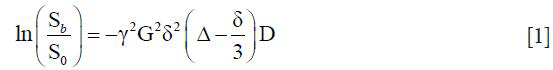
Where Sb and S0 are the echo signals in the presence and absence of the diffusion gradients, γ is the gyromagnetic ratio, G is the gradient amplitude, Δ is the gradient separation, δ is the gradient duration and D the diffusion coefficient. These parameters are usually combined into a single parameter known as the b-factor where:
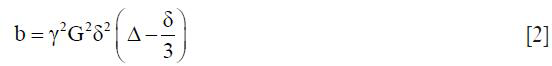
Thus, the sensitivity of the imaging sequence to water diffusion can be altered by changing the b value, or b factor. Increasing b value can be theoretically obtained by (I) increasing the strengths (heights) of the diffusion sensitizing gradients, (II) increasing their durations, and (III) increasing the gap between the paired gradient lobes. The signal intensity from protons with larger diffusion distances per unit time (e.g., blood flow associated pseudo-diffusion) is attenuated with small b values. By comparison, when higher b values (e.g., ≥500 s/mm2) are used, there is usually less signal attenuation from cellular tumors containing protons with shorter diffusion distances, compared with the normal liver. The echo signal in a typical spin-echo sequence (Figure 1) combines T2 and diffusion-weighting (with only negligible T1 weighting):
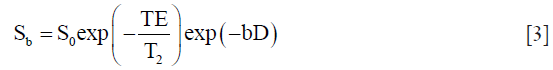
In order to remove the effect of TE on diffusion measurement, increasing b value is obtained by increasing the strength of the diffusion gradients in practice to keep the same TE value. As such, by measuring the signal at two different b values, the effects of T2 decay can be removed, leaving just the diffusion-weighted attenuation. By combining Eqs. [1-3], it is obtained that
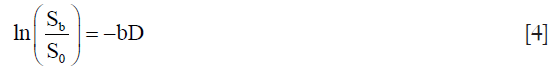
Thus it is able to calculate the diffusion coefficient D in each voxel of the image. A more accurate estimate can be obtained via linear regression with a series of DWI of different b values.
Using pure water at body temperature (37 °C) as a reference standard, the average displacement of water molecules during a 50-ms interval is approximately 30 µm (18). Because this is comparable to or greater than the dimensions of cells, there is a high probability that water molecules will interact with cells and their hydrophobic membranes and macromolecules will impede the motion of water. The observed or “apparent” diffusion of water within tissues is typically several-fold less than in pure water. Moreover, diffusion in biologic systems is affected by water exchange between intracellular and extracellular compartments and the tortuosity of the extracellular space (which in turn is affected by cell sizes, organization, and packing density). Thus, although the spatial resolution of DW-MRI is typically on the order of millimeters, DW-MRI is exquisitely sensitive to changes in diffusion measured on the cellular scale (e.g., micrometers). A clear example of the ability of DW-MRI to document directional diffusion from which architectural features can be derived is the anisotropy depicted in highly directional structures (e.g., myelinated white matter fiber tracts).
Although a number of DWI sequences can be applied to evaluate the liver, single-shot spin-echo (SE) echo-planar imaging (EPI) technique is the most frequently used in combination with fat suppression (e.g., spectral attenuated inversion recovery or chemical excitation with spectral suppression) (19-21). EPI samples all the k-space data points necessary to reconstruct the image using a gradient echo train after a single 90–180 pair of RF pulses (22). However, the maximum attainable spatial resolution of EPI can be limited by T2*-decay during the long duration of the gradient echo train. In addition, EPI has only a very small bandwidth per pixel along the phase encoding direction. Hence, EPI is very susceptible to off-resonance effects, such as main field inhomogeneity, local susceptibility variations, and chemical shift, which all may lead to severe image artifacts (22). To reduce such artifacts, diffusion-weighted single-shot EPI can be combined with parallel imaging like SENSE and/or other acceleration strategies. Single-shot SENSE-EPI reduces the train of gradient echoes in the EPI-readout leading to a faster k-space traversal per unit time. The resultant increased bandwidth per pixel in the phase-encoding direction and the shortened EPI train thus improve image quality. Imaging artifacts may also be ameliorated using other pulse sequences or alternative k-space trajectories (22).
All DW-MRI measurements are influenced by artifacts and machine imperfections. These include B0 inhomogeneity resulting from susceptibility variations within biologic or physical test objects/samples (this includes patients, volunteers, and nonhomogeneous structured phantoms). Chemical shift artifacts result from the presence of more than one chemical species or scalar coupling. Other artifacts are measurement-induced, for example, Nyquist ghosting and geometric distortions from residual motion-probing gradients (MPGs)-induced eddy currents.
Single-shot SE echo-planar DW MR imaging still has limited image quality, including poor SNR, limited spatial resolution, and EPI-related artifacts (mainly distortion, ghosting, and blurring) (23). 3T MRI has increased SNR, enabling higher spatial resolution compared with 1.5T. However, a fourfold increase in the SAR compared with 1.5T, higher sensitivity to susceptibility artifacts, B1 inhomogeneities and higher readout bandwidths were reported and in some cases, may significantly affect image quality. Uniform fat suppression for liver DWI has always been a challenge with 3T magnets and susceptibility artifacts are also more pronounced at 3T scanners. Promising strategies to obviate the disadvantages of 3T systems include the use of non-EPI sequences (turbo-FLASH, HASTE, SSFP) and dual-source parallel RF excitation DWI.
To ensure high-quality DW-MR images, the following summarizes the key factors that would help to optimize image quality (24).
- Parallel imaging is used in the body as this shortens echo-train lengths and reduces susceptibility and magnetic field inhomogeneity-related artifacts.
- Multiple averaging at high b-factor is used. To acquire additional averages at higher b value (e.g., >500 s/mm2) can be advantageous to compensate for reductions in SNRs at high b values.
- TR should be sufficiently long to avoid T1-saturation effect, which results in an underestimation of ADC values. The TE should be kept as short as possible because this results in better SNR and it minimizes motion and susceptibility EPI related artifacts. TE is typically 50–90 ms at 1.5T and even shorter at 3T. Tetrahedral encoding or other simultaneous application of gradient schemes (e.g., three-scan trace (Siemens), gradient overplus (Philips) should be used to achieve the shortest possible TE.
- Where available, use advanced or higher-order shimming techniques. Eddy currents related to diffusion gradients and EPI techniques lead to geometric distortions and image shearing, which can be reduced by increasing readout bandwidths or reducing the echo spacing, conversely reducing the length of image readout. For body imaging, this is typically 1 to 2 kHz per pixel. However, increasing bandwidths increases noise and Nyquist ghosting, and so bandwidths or echo spacing settings should be optimized.
- By reducing the amplitude of the higher b values either directly or by using three-scan trace methods (these generally reduce the amplitude of the individual gradients by a factor of 0.5–0.67 depending on vendor implementation).
Moreover, consider performing measurements in the fasting state to minimize air in the stomach, which may degrade images of the left liver.
ADC quantitation
When performing diffusion-weighted magnetic resonance imaging (DW-MRI) in the liver, it is advantageous to perform imaging by using both lower and higher b values (e.g., three b values, b=0, ≤100, and ≥500 s/mm2 (typically 500–750 s/mm2). Images with b value less than 100–150 s/mm2 nulls the intrahepatic vascular signal, creating the so-called black-blood images, which improves detection of focal liver lesions, while higher b values (≥500 s/m2) give diffusion information that helps focal liver lesion characterization. Additional b values can be considered when the primary aim is to obtain an accurate ADC since increasing the number of data points can reduce the error in the ADC estimation. Because of the relatively short T2 relaxation time of the normal liver parenchyma, the b values used for clinical imaging are typically no higher than 1,000 s/mm2. Liver signal is low when b value is greater than 800 s/mm2, and noise may contribute substantially to the signal and influence the calculation of diffusion coefficients. To generate b values larger than this would generally require the use of longer diffusion-gradient pulses with longer echo times and thus being prone to loss of signal from T2 decay.
ADC was introduced in 1986 (14), it is the most used diffusion parameter in liver. ADC (in mm2/s) is obtained by a mono-exponential fit of signal intensity function of b-value. Though most commercial software often performs mono-exponential regression with ≥2 b values, the ADC is most commonly calculated by mono-exponential regression using two b values with the formula:

where SIb1 and SIb2 denote the signal intensity acquired with the b-factor value of b=b1 and b=b2 s/mm2, respectively.
The value of the ADC strongly depends on the b values chosen for its calculation. ADC is overestimated when b=0 s/mm2 is included to calculate it because the effect of perfusion is also incorporated in the calculation (see the IVIM paragraphs below) (Figure 2). Another problem of ADC quantitation is the DW images’ signal can be much affected by noise. Even the same two b values are chosen, the reproducibility can be problematic. For b values >50–100 s/mm2, signal attenuation can be considered mono-exponential, and ADC calculated with b >50 s/mm2 as the first value (and not b=0) is more reproducible (25) .

It should be noted that as a malignant liver tumor can have both restricted water motion and in the meantime increased perfusion. For ADC computed including b=0 images, these two effects in the opposite directions may cancel each other to various extents, thus ADC becomes a less sensitive biomarker. However, it is recommended to acquire the nominal b=0 image to provide anatomic information. Usually, the b=0 image can be obtained quickly using single-shot techniques, because acquisition along three-orthogonal axes is not performed for the b=0 weighting. It is possible to fractionate the calculation of the ADC if three or more b values are used at DW MR imaging. For example, if DW imaging is performed by using three b values of 0, 100, and 500 s/mm2, it is possible to calculate the ADC by using all three b values. However, it is also possible to calculate a perfusion-insensitive ADC by using just the higher b values (100–500 s/mm2) or a perfusion-sensitive ADC by using the lower b values (0–100 s/mm2). For clarity, the b values used to calculate the ADC can be systematically included after the term “ADC”, For example, if b values of 50, 200 and 400 s/mm2 are used to calculate the ADC, the ADC can be cited as “ADC (b=50, 200, 400)” (25).
Note the signal intensity observed on the diffusion image is dependent on both water proton diffusivity and the tissue T2-relaxation time. This means that a lesion may appear to show restricted diffusion on DW MR images because of the long T2-relaxation time rather than the limited mobility of the water protons. ‘T2-shine through’ is the term to describe hyper-intensity of tissues related to the intrinsic T2-weighting of DW images and to be present when mild hyperintensity is seen on high b value images (800–1,000 s/mm2) and on ADC maps. This phenomenon can be observed in the normal gallbladder, cystic lesions, and hemangiomas (Figure 3). Areas demonstrating substantial T2 shine-through rather than restricted diffusion will show high diffusivity on the ADC map and high ADC values.

The ADC values for all voxels can be displayed as a parametric map. Both region-of-interest and histogram analysis of ADC measurement can be obtained. For drawing ROI, the b=0 (or a very low b value image) is usually used, although high b value images may also be used. In the latter, it should be noted that high b value images may be associated with more severe image distortion. If traditional anatomic images, which are independent of the DW-MRI sequences, are used to draw ROI, then image registration is required, as DWI images are more likely to suffer from distortions.
Note ADC quantification requires minimum acceptable SNR at higher b values. Use of low-SNR images for ADC quantification may negatively affect ADC quantification reliability. Low SNR pixel values can be eliminated before the ADC map calculation, and these pixels can be flagged as “not-a-number” for the exclusion (24). In tumor assessment, the inclusion of necrotic and cystic zones can include extremes in water ADC values, which may bias image analysis.
ADC values (thus also IVIM measurement) have been reported to be influenced by the presence of fat or iron within the liver. Liver tissue with high iron concentration is associated with decreased ADC measure (26).
Applications of liver DW-MRI
The ease of acquisition and ability to obtain perfusion and diffusion information without the necessity of intravenous contrast administration have contributed to the growing interest in exploring clinical applications of DW-MRI. DW-MRI can be quick and performed within a breath-hold and it can be readily incorporated to existing protocols.
Applications of liver DW-MRI: liver lesion detection
DW-MRI improves sensitivity in the detection of focal lesions, helps tissue characterization (differentiating benign from malignant lesions), support monitoring treatment response and differentiating post-therapeutic changes from the residual active tumor as well as detecting recurrent cancer. DW-MRI can be included in routine liver MR protocols in combination with conventional unenhanced and contrast-enhanced MRI. It is usually performed prior to contrast agent administration, although performing DW-MRI after the Gadolinium administration may not affect DW-MRI assessment. DW images should be interpreted concurrently with the ADC map and all other available morphologic imaging.
Cellular tissues, such as tumors, demonstrate restricted diffusion (high signal intensity) on higher b value (≥500 s/mm2) images and low ADC value. By contrast, cystic or necrotic tissues will show a greater degree of signal attenuation on higher b value diffusion images and have higher ADC value. The reason(s) why malignant tumors have lower ADC values are poorly understood but is probably related to a combination of higher cellularity, tissue disorganization, and increased extracellular space tortuosity, all contributing to the reduced motion of water (24). DW-MRI at high b values (≥100 s/mm2) also provide a low background signal from normal liver parenchyma and thereby results in increased contrast between the background liver and lesions, enhancing the detection of focal liver lesions (Figures 4,5,6).


Studies comparing DW-MRI and T2 weighted sequences generally show better performance of DW-MRI. DW-MRI is especially useful in the detection of small lesions around vessels and in the periphery of liver, which can be challenging to detect on routine T2 weighted images. DW-MRI adds value in oncologic patients by depicting more liver lesions when combined with contrast-enhanced MRI protocols, and improves reader confidence in lesion detection, particularly for small tumors (28-31).
Due to ‘T2-shine through’, tissues with long T2-relaxation time show hyper-intensity on DW images and ADC maps (Figures 3,7).

Applications of liver DW-MRI: liver lesion characterization
In general, tumors have lower ADC value, whereas normal/benign/reactive tissues have higher ADC value with a variable degree of overlap. Malignant lesions such as HCC and liver metastases usually display low ADC values, except when treated and/or necrotic. Focal nodular hyperplasia (FNH) and adenomas have intermediate ADC value that can overlap with those of malignant lesions and normal liver parenchyma. ADC values for distinguishing malignancy from normal/reactive tissues and benign disease depend on histologic characteristics such as tumor type, differentiation, and necrosis.
In malignant lesions, DW-MRI is useful in distinguishing the different components of tumors (cystic and/or necrotic vs. solid components). Hyper-intensity on high b value DWI associated with lower ADC value suggesting active tumor. Tumor necrosis corresponds to higher ADC values compared with viable tumor. Hepatic metastases that demonstrate substantial central necrosis can demonstrate high ADC. Mucinous malignant lesions that may show a lower restriction to diffusion and high ADC and can be misdiagnosed as benign lesions.
Liver cysts show pronounced decrease in signal intensity with increasing b values and the highest ADC values, followed by hemangiomas. The microscopic presence in hemangiomas of cellular components, such as endothelium, fibrous tissue, and blood, resulting in restricted diffusion compared with other cystic lesions with a more complete fluid content.
The diagnostic performance of DW-MRI reported in the study by Parikh et al. (32) [area under the curve (AUC), sensitivity, and specificity of 0.839, 74%, and 77%, respectively] likely reflects the realistic diagnostic performance of ADC for various liver pathologies.
ADC value correlates with histopathological differentiation and microvascular invasion with poorly differentiated HCCs showing lower ADC than well-differentiated and moderately differentiated HCCs (33-36). Heo et al. (36) described that all iso- to hypovascular lesions on gadolinium-enhanced examinations, which were also visible on DW-MRI were poorly differentiated HCCs, whereas lesions not visible on DW-MRI were low-grade HCCs or dysplastic nodules. The recurrence-free survival was found to be shorter in low-ADC group than in high-ADC group (34). Because HCCs often contain a few components with different histological grades, their DWI appearances are often inhomogeneous, so Nishie et al. (37) suggested measuring minimum ADC so to detect the worst histological grade of the tumor.
Catalano et al. (38) described that, in patients with locally advanced HCC, DW-MRI was useful in characterization of the venous thrombus as bland vs. tumor thrombus. The mean ratio of the ADC of the thrombus to the ADC of the tumor in the bland thrombus group was 2.9 compared with 0.998 in the neoplastic group.
DW-MRI in assessment of tumor response to treatment
DW-MRI is increasingly applied to evaluate tumor response to various therapies including biologics therapy, chemotherapy, radiation therapy, and local ablation. Generally speaking, effective tumor treatment results in an increase in the ADC value, which can occur prior to a measurable change in tumor size (24,39-41) (Figure 8). Higher ADC value likely represents post-therapeutic extracellular edema, whereas lower value parts are suspicious for active disease. An increase in ADC values following systemic chemotherapy can be a sign of tumor response with non-responders showing lower ADC values than responders (42,43).

However, a transient ADC decrease phase within 24–48 hours after initiation of treatment has been observed; which may be related to cellular swelling, reductions in blood flow, or reduction in extracellular space (24,44).
Following the increase in ADC with treatment, the ADC can eventually decrease, which is related to tumor repopulation and fibrosis.
For a rigorous prospective study assessing treatment response, double-baseline scans, i.e., to perform baseline examination twice, will be valuable as this provides data about measurement error of imaging specific to the study and thus provides information of what constitutes a significant change in an individual and a group of patients (24).
Liver cirrhosis with DW-MRI
There is sufficient evidence that liver cirrhosis is associated with lower ADC measurement (45-47). The mechanism of diffusion restriction in liver cirrhosis fibrosis is multifactorial and not completely understood, but possibly related to the presence of increased connective tissue in the liver, which is proton poor, and decreased blood flow. However, it can also be concluded that at present, simple ADC measurement cannot replace liver biopsy for liver fibrosis assessment (48,49). ADC is not sensitive for early-stage liver fibrosis.
As both HCC and cirrhosis have decreased ADC, thus in some cases HCCs may become difficult to differentiate from surrounding cirrhotic changes or dysplastic nodules.
Fatty liver and DW-MRI
The presence of fat within the liver is associated with lower ADC measure (26). The histologic features of non-alcoholic fatty liver disease (NAFLD) and steatosis is correlated with decreased ADC, which has been shown both in human and animal studies (49,50).
Technical aspects of intravoxel incoherent motion (IVIM) analysis
In the traditional diffusion theory, the movement freely mobile water molecules diffusing from one location to another in a certain time is considered to have a Gaussian distribution. Based on this Gaussian diffusion behavior, a mono-exponential decay function of DWI signal intensity with regard to the increase of b value has been adopted for diffusion analysis (15,16). However, water diffusion behavior in biological tissues is more complicated than the completely free water diffusion in space due to the complex cellular structures of tissues with many diffusion barriers like membranes. Consequently, the displacement probability of tissue water may substantially deviate from a Gaussian form and hence violates the validity of the monoexponential model to varying extents depending on in-vivo tissue characteristics. Several non-Gaussian diffusion models have been proposed to account for the non-Gaussian diffusion behavior of biological tissues (51-56). These non-Gaussian diffusion models were mostly proposed and applied for brain DWI initially, while their applications to other tissues have been increasing in recent years. By considering the continuous distribution of microscopic diffusion compartments attenuating at different rates with b-values, stretched-exponential model (SEM) (54) and statistical diffusion model (SDM) were proposed (53). Besides, diffusion kurtosis imaging (DKI) model used the Taylor expansion of the DWI signal attenuation in powers of b value to measure the excess diffusion kurtosis in addition to the diffusion coefficient (52). These different non-Gaussian diffusion models may reveal different aspects of tissue properties.
IVIM bi-exponential analysis
As the most tested example of Gaussian diffusion model, IVIM was proposed by Le Bihan et al. (15,55,56) to account for the effect of capillary perfusion on the aggregate DWI signal. Two separate parameters (along with their volume fractions) have been proposed to reflect the true tissue diffusivity and capillary perfusion, respectively, in the mathematical form of a bi-exponential decay function. According to IVIM theory, the fast component of diffusion is related to micro-perfusion, whereas the slow component is linked to molecular diffusion. The signal decay of IVIM diffusion MRI is therefore described with a bi-exponential model (15).

where SI(b) and SI0 denote the signal intensity acquired with the b-factor value of b and b=0 s/mm2, respectively. The perfusion fraction (PF, or f) represents the fraction of the pseudo-diffusion compartment related to microcirculation, Dslow (or D) is the diffusion coefficient representing the slow (pure) molecular diffusion, and Dfast (or D*) is the pseudo-diffusion coefficient representing the incoherent microcirculation within the voxel (perfusion-related diffusion).
The bi-exponential decay behavior of signal intensity on MR image and b-factor can be analyzed with segmented fitting or full fitting. For the segmented fitting, the signal value at each b value is normalized by attributing a value of 100 at b=0 s/mm2 [Snorm =(SI / SI0) × 100, where Snorm is the normalized signal, SI=signal at a given b value, and SI0=signal at b=0 s/mm2]. The estimation of Dslow is obtained by least-squares linear fitting of the logarithmized image intensity at the b values greater than a threshold b-value (such as 200 or 60 s/mm2) to a linear equation. The fitted curve is then extrapolated to obtain an intercept at b=0. The ratio between this intercept and the SI0, gives an estimate of PF. Finally, the obtained Dslow and PF are substituted into Eq. [6] and are non-linear least-square fitted against all b values to estimate Dfast. With the full fitting method, all the parameters (Dslow, Dfast, PF) are estimated by a single least‐squares nonlinear regression.
Typically, for healthy liver and bi-exponential fitting starting from b=0, Dslow is around 1.0×10⁻³–1.1×10⁻³ mm2/s, PF is around 18–22%; Dfast value can vary more widely, ranging from 40×10−3 to 100×10−3 mm2/s or even more. These values are also affected by how ROI is drawn. With ROI including more vessel pixels, IVIM parameters increase. Furthermore, the value of three IVIM parameters derived from IVIM analysis depends on the b value distribution, the fitting method, as well as the threshold b value for segmented fitting. For the segmented fitting, a higher threshold b value is associated with flatter Dslow curve (i.e., lower Dslow value) and leads to higher PF measurement. A lower threshold b value leads to Dslow curve containing more perfusion compartment, and therefore higher Dslow measurement and lower PF measurement (Figure 9). Only including low b values which correlate to the initial sharp signal decay lead to higher Dfast measurement (57,58). Note the dependence of PF, Dslow, and Dfast on threshold b value differs between healthy livers and fibrotic livers; with the healthy livers showing a higher degree of dependence (57).

Segmented fitting remains an approximating approach that emphasizes the accuracy of Dslow estimation while allows less flexibility for Dfast calculation. For bi-exponential model, full fitting provided better fit at very low and low b-values compared with the segmented fitting with the later tended to underestimate Dfast; however, the segmented method may have a lower error in signal prediction for high b values (58) (Figure 10). Theoretically, full fitting shall allow more flexibility and therefore the possibility to produce results closer to the true physiological value of IVIM parameters. However, the segmented fitting approach has commonly been used since the simultaneous fitting of all diffusion parameters usually gives less stable results (58,59).

Tri-exponential IVIM
Compared with the bi-exponential model, earlier work of Cercueil et al. demonstrated that a third very fast diffusion compartment may exist (60). More recently, Wurnig et al. also demonstrated the presence of a third component of diffusion in liver and kidney (61). Chevallier et al. (58) demonstrated that bi-exponential model cannot fit correctly very low (range: 3–10 s/mm2) and low b values (range: 25–80 s/mm2) at the same time, which particularly lead to inaccuracy in Dfast estimation. Tri-exponential model provides a better fit for IVIM signal decay in the healthy liver than the classical bi-exponential model (Figure 11).
For tri-compartmental model, the signal decay is modeled according to the following Eq. [7]:
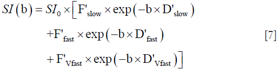
Where D’slow represents the diffusion coefficient thus being similar to Dslow, D’fast and D’Vfast represent the fast and very fast perfusion-related pseudo-diffusion coefficients. F’slow, F’fast, and F’Vfast are the fractions of each compartment. F’slow is similar to the fraction of the slow diffusion compartment (1 − PF) and the combination of F’fast + F’Vfast is similar to PF of the bi-exponential model. (F’Vfast =1 − F’slow − F’fast) can be assumed to simplify the Eq. [7] with 5 rather than 6 parameters (58,60).
For tri-exponential model, the difference between full fitting and segmented fitting tends to be small concerning the fitting quality (Figure 11), while segmented fitting is preferred due to its better scan-rescan reproducibility (i.e., fitting stability) (58). The more coefficients are added to a model, the more likely estimated parameters become less stable (58).

Earlier work of Gurney-Champion et al. (62) proposed the removal of voxels presenting high ADC value on ADC image created from b=0 and 10 s/mm2, i.e., the removal of voxels presenting tri-exponential decay. Gambarota et al. (63) proposed to first detect the number of the compartments by using non-negative least squares method and then to process the fit without b=0 data point in pixels presenting a tri-exponential decay. However, in Chevallier et al.’s work (58), ROI-analysis was used and the results suggest that the majority of pixels included in the ROI showed a tri-exponential behavior. Indeed, it can be shown that even when ROI is drawn on liver parenchyma to exclude bright pixels which would contain ‘visible’ vessel, a sharp drop of signal from b=0 to b=2 can still be seen, suggesting the inability of a bi-exponential model to fit the signal decay at very low b values (unpublished data, YX Wang, N Che-Nordin, H Huang) (Figure 12).

IVIM bi-exponential fitting without b=0
The signal difference between b=0 s/mm2 image and b=1 or b=2 s/mm2 images can be very substantial, the vessels (including small vessels) particularly show high signal without diffusion gradient while showing dark signal when the diffusion gradient is on even at b=1 s/mm2. With most of the reported IVIM analyses, the diffusion image signal decay is computed starting from b=0 s/mm2 image and then increasingly higher b values using a bi-exponential decay model. However, this decay process may not follow the bi-exponential model for ROI (region-of-interest) based analysis. While, due to the respiratory motion and low signal-to-noise ratio, we favor ROI-based analysis for liver IVIM as opposed to voxel-wise analysis. Respiratory motion is likely to cause voxel misalignment in the Z-direction. We propose that the relationship between liver DWI signal and b value can be separated into two parts: part-1 is the signal difference between b=0 image and the first very low b value image (usually b=2 image), and the rest is part-2 and fitted with bi-exponential decay (64-67). For this part-1, we propose that liver vessel density can be measured by a DWI derived surrogate biomarker (DDVD): DDVD/area(b0b1) = Sb0/ROIarea0 − Sb1/ROIarea1 or DDVD/relative = (Sb0 − Sb1)/Sb1, where Sb0 refers to the measured liver signal intensity when b=0 s/mm2, and Sb1 refers to the measured liver signal intensity when b=1 s/mm2. This Sb1 can also be replaced by Sb2 or even Sb10 (measured liver signal intensity when b=2 s/mm2 or b=10 s/mm2). Of note, the sharp signal decay between b=0 image and image of very low non-zero b value does occur in liver parenchyma parts where no vessels can be visible with MR imaging (Figure 12). This is due to the rich micro-circulation being imaged; while due to intrinsic spatial resolution limitation of MRI, vessels of sub-millimeter cannot be visualized by MRI.
For bi-exponential decay analysis with b=2 s/mm2 image as the starting point, the signal value at each b value is normalized by attributing a value of 100 at b=2 s/mm2 [Snorm=(SI/SI2)×100, where Snorm is the normalized signal, SI=signal at a given b value, and SI2=signal at b=2 s/mm2]. The signal attenuation is modelled according to Eq. [8]:

Where SI(b) and SI2 denote the signal intensity acquired with the b-factor value of b and b=2 s/mm2.
IVIM b value selection and image post-processing
Due to its relatively high blood supply, the liver is a very suitable organ for IVIM analysis. However, the liver is in the meantime particularly affected by physiological motions such as respiration and heart beating; the left liver is also affected by susceptibility artefact due to contents in the stomach. IVIM diffusion imaging was for one period considered to be very difficult to implement in the liver. Scan-rescan reproducibility can be unsatisfactory for quantification of the perfusion related fast compartment of Dfast and PF (perfusion fraction), while Dslow may not be sensitive to pathological change (68-73). In a systematic review conducted in 2016, it was concluded that the literature till then showed liver IVIM was not able of detecting early-stage liver fibrosis and diagnosing liver fibrosis grades, nor can it differentiate liver tumors (68).
Recently it was demonstrated that, with sufficient and improved selection of b values and careful image post-processing, PF and Dslow measurements can be quite reproducible, and Dfast can be moderately reproducible (58,74). Generally, more b values will improve fitting stability (68). Ter Voert et al. (70) recommended 16 b values for liver IVIM study, and this is the number of b values we have been using in recent years (58,66,67,74). With current MRI technology, multiple slices covering the whole liver can be obtained with respiration-gating and 16 b values in approximately 5 min. Moreover, for standard clinical MRI scanner of current technology, b value ≥800 s/mm2 may be substantially affected by noises, and may not be suitable for liver parenchyma DWI assessment (Figure 13). We also recommend discarding liver IVIM image series with substantial respiratory motions and poorly fitted curves (74). During the image post-processing, it is critically important to check the quality of the fitting curves before adopting the results of fitted results (Figure 14). When drawing an ROI, it is also important to avoid parts with artifacts or very low SNR (Figure 15). With free-breathing or respiratory-gating, human volunteers and patients should be comfortably secured within the magnet and their breathing well trained to keep regular shallow breathing during image acquisition. As post-meal and fasting status may influence the blood flow to the liver, it can be recommended that patients fast for 6 hours before liver IVIM DWI.


With bi-exponential full fitting, the perfusion related fast compartment is estimated to contribute for around 17% of the total signal at b=0 s/mm2, then decreases to become negligible at b≥25 s/mm2 (58). Thus, the commonly used threshold b value of 200 s/mm2 to separate fast component and slow component may be too high. When b=0 image was not included for bi-exponential decay fitting, we also empirically showed that, as compared with the commonly used threshold b-value of 200 s/mm2, the threshold b value of 60 s/mm2 to separate Dfast and Dslow performed better in separating normal livers and fibrotic livers (57,66,67).
Three b value IVIM analysis
Some researchers described three b values technique to obtain Dslow and PF, while generally ignore Dfast as it could not be reliably estimated with three b values. If images of three b values can be acquired in a single breath-hold, then voxel-wise parametric maps of Dslow and PF can be generated; this will allow a visual assessment of heterogeneous lesions and the targeted quantitative analysis of necrotic or viable areas for tumor. Mürtz et al. and Penner et al. reported that the approximation of Dslow and PF from b=0, 50, 800 s/mm2 was superior to that from b=0, 250, 800 s/mm2 (within a given scan time) and provided more discriminatory power between different lesion groups than conventional ADC from b=0, 800 s/mm2 (75-77). This is understandable since the perfusion contribution at b=250 s/mm2 is already very low. Regarding the differentiation between malignant and benign lesions, good differentiability between malignant and benign lesions was found in studies where the benign lesion group included cysts or consisted of haemangiomas (both are lesions with high ADC and high Dslow values). However, their results revealed a tendency towards a lower PF in malignant lesions, which does not agree with most of the other studies. Of note, the number of excitation (NEX, or number of signal averaging) was not reported in their studies (75-77).
Murphy et al. (49) described more details with their three b value IVM method. They acquired multiple single excitation images, with 8, 16, and 32 repetitions at b=0, 100, and 500 s/mm2, respectively. Total imaging time was 2.8 minutes. Patients were instructed to breathe freely during the acquisition, without cardiac or respiratory gating.
Single-breath-hold IVIM image series acquisition
Currently, IVIM data series have been acquired with free-breathing or respiratory-gating, both approaches are still associated with respiratory motion. Thus, single-breath-hold IVIM image series acquisition may be advantageous (Figure 16). The feasibility of single-breath-hold has been preliminarily demonstrated (Figure 17) (64). In our testing (unpublished data, O Chevallier & YX Wang), MR imaging was performed with a 3T magnet equipped with a dual transmitter. The IVIM DW imaging sequence was based on a single-shot DW spin-echo type EPI sequence, IVIM imaging parameters included pixel size =3×3 mm, slice thickness =15 mm, TR=104 ms, TE=45 ms, flip angle=90°. b=1 (dummy scan, NEX=1), 0 (NEX=1), 10 (NEX=1), 20 (NEX=1), 40 (NEX=1), 60 (NEX=1), 80 (NEX=1), 100 (NEX=1), 150 (NEX=1), 200 (NEX=2), 400 (NEX=2), 800 (NEX=3) s/mm2. SPIR technique was used for fat suppression. The breath-hold duration was 14 s.


We have developed experiences with our past work on breath-hold MRI image acquisition (78,79). Breath-hold should be trained for the scan subjects before the scan starts. It is more likely that the diaphragm and liver position would shift during the breath-hold period if a subject holds his/her breath after full end-inspiration or full end-expiration. Therefore, the scan subject should be asked to hold his/her breath during usual-depth breathing. After hearing the ‘hold-breath’ instruction, the subject should be given sufficient time to allow the diaphragm back to the most comfortable position. Therefore, a time delay is allowed between the scan operator to give ‘hold-breath’ instruction and to push the MR data acquisition start button so that the scan subjects will have time to react to the ‘hold-breath’ instruction. The respiration-gating balloon is placed on the top of the scan subjects’ upper abdomen, and the quality of the ‘breath-hold’ is monitored on the respiration-triggering screen on the MRI console. A repeatability study is shown in Figure 18, where a healthy volunteer was scanned for 6 times during a single session when the data acquisition parameters and slice selection remained the same.

Till now, there are several limitations for this technique. To achieve the desirable total b value number of 16 (64), longer breath-hold (>14 s) is required which will be beyond the tolerability of most patients. The SNR remains not optimal. Moreover, it is a single slice acquisition, though multiple slices can be obtained with multiple breath-holds.
Multi-exponential analysis
Living tissues exhibit multi-exponential signal decay over a broad range of b values. Even after the elimination of perfusion effects, tissues can still exhibit multi-exponential signal decay at very high b values (b=1,000–5,000 s/mm2). Analysis of these data types requires multi-exponential models where signal decays are modelled as weighted sums of two or more exponentials (80,81), or alternative models such as stretched exponentials that allow distribution of diffusion coefficients (54). For liver, these models are typically applied to liver tumors, with their highly restricted water motion and slow signal decay at high b values. However, as noted above, for normal liver tissue, SNR can be very low for images with b value >1,000 s/mm2.
Some interesting studies using multi-exponential analysis have been reported. For example, Wang et al. (82) reported that mean kurtosis was correlated with MVI (micro-vessel invasion) and could yield better predictive accuracy for MVI than ADC. Recently, Cao et al. (83) reported that diffusion kurtosis imaging-derived mean apparent kurtosis coefficient (MK) values outperformed conventional ADC values for predicting MVI and histologic grade of HCC. MK was significantly higher in MVI-positive than in MVI-negative group; high-grade HCCs showed significantly higher MK values than low-grade HCCs; higher MK and Barcelona Clinic Liver Cancer stage C were independent risk factors for early HCC recurrence (83). A more detailed discussion of non-Gaussian analysis is beyond the scope of this review. Overall, when a very high b value is applied, it is critically important to assess the SNR of the DW images before performing curve-fitting procedures.
Clinical applications of liver IVIM imaging
IVIM technique has been investigated in a number of clinical applications, most notably in liver fibrosis, NAFLD and NASH, and liver tumors.
Applications of IVIM in liver fibrosis
The result of untreated chronic viral hepatitis is inflammation, loss of liver parenchyma, and healing by fibrosis and regeneration. Liver fibrosis is characterized by the extracellular accumulation of collagen fibers, glycosaminoglycans, and proteoglycans, which result in restricted water diffusion. In subjects with liver cirrhosis, arterial and portal venous pressure increase; additionally, intrahepatic and extrahepatic portal venous shunts reduce vascular liver input, leading to decreased micro-perfusion.
Earlier works suggested liver fibrosis is more associated with fast compartment (Dfast and PF) reduction than Dslow reduction. Luciani et al. (84) applied the IVIM model to quantify PF, Dslow, Dfast, and ADC of normal and cirrhotic liver parenchyma. They found significantly lower Dfast and ADC in cirrhotic livers, but no difference in Dslow between normal and cirrhotic livers. In their case, since b=0 images were included to compute ADC, their ADC thus contain perfusion component. In a rat model of diethylnitrosamine-induced liver fibrosis, Zhang et al. (85) reported that PF values decreased significantly with the increasing fibrosis level; but Dslow was poorly correlated with fibrosis level. Annet et al. (86) showed that rats with hepatic fibrosis demonstrated reduced ADC values in vivo but not when DW MR imaging was performed ex vivo, which favors the perfusion effect on diffusion measurement. Our data shows, among the three IVIM parameters, PF was the most responsive to liver fibrotic changes, probably due to that, the Dfast remains difficult to be estimated precisely (65-67). As can be expected, Dfast and PF are positively correlated; while a correlation between Dslow and the fast component (Dfast or PF) was not shown (66).
The most encouraging results till now are probably those published by Wáng et al. (65), Huang et al. (66), and Li et al. (67) (Figures 19,20). Wáng et al.’s report had 16 healthy volunteers and 33 hepatitis B liver fibrosis patients, among them 15 patients had stage-1 liver fibrosis. Huang et al.’s report had 26 healthy volunteers and 12 hepatitis B liver fibrosis patients, among them 4 patients had stage-1 liver fibrosis. Li et al.’s report had 20 healthy volunteers and 28 hepatitis B liver fibrosis patients, among them 11 patients had stage-1 liver fibrosis. All patients and healthy volunteers can be separated by IVIM analysis except one stage-2 fibrosis case in study-3. Interestingly, Huang et al.’s study and Li et al.’s study both had 4 patients respectively with biopsy showing no fibrosis, and these 8 subjects’ diffusing MRI measurements resembled healthy volunteers.


Applications of IVIM in NAFLD and NASH
NAFLD is defined by the deposition of lipids within hepatocytes in the absence of substantial alcohol intake. Approximately 20% of patients with NAFLD have a progressive form of the condition known as nonalcoholic steatohepatitis (NASH), which is characterized by the presence of inflammation and hepatocellular injury in addition to steatosis. Patients with NASH may develop fibrosis and can progress to cirrhosis. NAFLD is the most common liver disorder in western industrialized countries with a prevalence of 6–35% worldwide (87). NASH can progress to cirrhosis in 15% of the patients (88).
Currently, there is an agreement that steatosis is associated with lower Dslow (49,89,90). The decrease in diffusivity associated with steatosis can be caused by two ways. Intracellular lipid restricts diffusion of water within hepatocytes. The second possibility is that lipid peaks near water are incompletely suppressed by the chemical shift-dependent suppression techniques used by the DWI sequence. If so, the measured diffusivity may incorporate the diffusion constant of lipid, which is two orders of magnitude slower than water (49,91).
Moreover, NASH and fibrosis are likely associated with reduced PF and Dfast. Murphy et al. reported that steatosis was associated with reduced Dslow and fibrosis with reduced PF (49). In an animal model, Joo et al. (92) reported that PF was significantly lower in rabbits with NAFLD than in those with a normal liver, and it decreased further as severity of NAFLD increased, with medians of 22.2%, 14.8%, 11.3%, and 9.5% in the rabbits in the normal, NAFLD, borderline, and NASH groups, respectively. Shin et al. (93) studied 123 children with 8 in the normal group, 93 in the fatty liver group, and 22 in the fibrotic liver group. They reported that Dfast value was lower in the fibrotic liver group compared with those of the normal and fatty liver groups. The PF value was lower in the fibrotic liver group compared with the fatty group. The Dslow and ADC values were not responsive for fatty liver and fibrotic liver changes (93). In 59 type 2 diabetic patients, Parente et al. (94) reported that both NASH and fibrosis were associated with lower Dslow and lower Dfast.
For analysis for diffused liver disease, we favor ROI analysis to cover a large portion of liver parenchyma while avoiding vessels. With this approach, the IVIM parameters are calculated based on the mean signal intensity of the whole ROI, which offer better estimation than pixel-wise fitting when the signal-to-noise of the DW images is low.
Applications of IVIM in liver tumors
While due to the technical differences in data acquisition and image post-processing, different results have been reported, some clear trends are still evidential in literature for IVIM’s application in liver tumor assessment (95-102).
Woo et al. (95) reported that Dslow and ADC are negatively correlated with HCC histologic grade. Dslow and ADC values were both significantly lower in high-grade HCC than in low-grade HCC. This trend was better shown with Dslow than with ADC (Figure 21A). PF was positively correlated with HCC’s arterial enhancement (95), and high-grade HCCs had higher PF values compared with the low-grade HCC group (96,97). In a recent study, Wei et al. (101) reported that reduced ADC and Dslow were related to MVI of HCC at univariate analysis; while at multivariate analysis, only Dslow value was the independent risk factor for MVI of HCC. Choi et al. (98) reported similar PF for HCC and metastasis, but intrahepatic cholangiocarcinomas had lower PF (Figure 21B). Compared with intrahepatic cholangiocarcinomas, HCC tends to be more hypervascular, which may explain a higher PF value for HCCs than for intrahepatic cholangiocarcinomas. PF correlate with the extent and degree of hepatic nodule enhancement in the arterial phase (98,99).

Klauss et al. (100) reported FNH has higher Dslow and ADC than HCC, indicating FNH’s benign nature as compared with HCC. Moreover, both Klauss et al. (100) and the Universitätsklinik Bonn group (75,76) reported higher PF in FNH than HCC.
In simple terms, it can be summarized that malignant liver tumors are associated with restriction water motion and thus lower Dslow, the increased blood supply to the malignant tumor neo-vasculature is shown with higher fast compartment measure (higher PF or/and higher Dfast). As compared with ADC and Dslow, it has also been shown that PF is a more responsive marker of sorafenib treatment in HCC (102). This observation concurs with the liver fibrosis studies (65-67), where PF is the most responsive parameter to fibrosis. Of note, for all pathologies, it is more likely that PF and Dfast change in the same direction (i.e., both increase or both decrease), as intuitively and evidently PF and Dfast are correlated (66). In cases when PF and Dfast change in opposite directions, measurement reliability should be double-checked.
Overall, reliable differentiation and the associated cut-off values of liver tumors by diffusion-IVM have not been established. Many published studies might have suffered from insufficient b values and suboptimal fitting stability. Previous reports of the differentiation power of diffusion-IVIM analysis, as well as good AUCs, have been partially due to the inclusion of cystic tumors such as hemangiomas. Cyst and hemangiomas can be most readily diagnosed with routine techniques, with a confirmative diagnosis made by the administration of contrast agent in selected cases.
DCE MRI
In liver DCE-MRI study, a series of liver T1-weighted images (phases) are acquired before, during, and after a bolus of contrast agent injection. Then the temporal change of the acquired images, reflecting the pharmacokinetics of contrast agent in liver, are analyzed with or without pharmacokinetic modelling techniques to generate quantitative or semi-quantitative parameters, which reflect the perfusion and/or hepatocyte function of the liver. Although DCE-MRI has not been widely used in clinical routine, many preliminary studies investigated its application in evaluating the response or predicting the outcome of treatments in various liver diseases, especially in liver tumors (103-109). This section briefly introduces the liver DCE-MRI techniques, including the contrast agents, acquisition methods and analysis techniques in liver DCE-MRI.
The basic theory of liver DCE-MRI
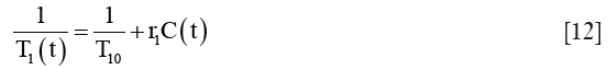
DCE-MRI is composed by a series of T1W to acquire the contrast agent concentration of the tissue during the contrast agent pharmacokinetics. The paramagnetic properties of gadolinium accelerate longitudinal magnetic relaxation process, thereby shortening T1 value of blood and tissue according to the following equation (110):
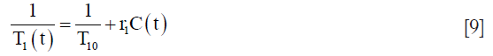
where T10 is the pre-contrast T1 value in the absence of the agent, C(t) is the contrast concentration. r1 is the relaxivity, whose value depends on the contrast type, magnetic field strength, solvents and temperature (typically 3–5 L·mmol−1·s−1) (110). The T1-shortening effect of contrast agent results in signal intensity increase on T1-weighted images. Thus, the temporal signal enhancement of the liver tissue reflects the pharmacokinetics of the contrast agent in the tissue. Then, the perfusion characteristics, even hepatocyte function of the liver tissue can be quantified using model-free (semi-quantitative) and model-based (quantitative) analysis.
The model-based analysis is based on the pharmacokinetic models, which describe the pharmacokinetics of injected contrast agent using compartment models. After venous bolus injection, the gadolinium-based contrast agents extravasate from intravascular (usually through dual pathways) to the extravascular extracellular space (EES), even into hepatocytes (only for mixed extracellular hepatobiliary contrast agents). Thus, an example pharmacokinetic model with commonly used extracellular contrast agent is as following (111):

where Ct represents the contrast concentration change of liver tissue. The CP and Ca are the contrast concentration change in portal vein and hepatic artery (usually can be extracted from aorta), respectively, and were named as vascular input functions [VIFs, including portal vein input function (PIF) and arterial input function (AIF), respectively]. Tp and Ta represent the transit time from the portal vein and aorta to the liver. ⊗ denotes the convolution operator. Thus, this model can be fitted with these two important VIFs and the contrast concentration curve of liver tissue to determine the perfusion parameters: portal blood flow Fp, arterial blood flow Fa and outflow rate K0 in this example model. In normal liver, approximately 75% of blood is provided by the portal vein [Fp/(Fa+Fp)=75%] and the left 25% through the hepatic artery (Fa/(Fp+Fa)=25%) (112). Under pathological conditions, especially in tumor, these perfusion parameters of liver tissue would change, which present the opportunities for DCE-MRI for liver disease evaluation.
Contrast agents
There are two major types of clinically available contrast agents used in liver DCE-MRI: (I) extracellular gadolinium-based contrast agents, such as gadopentetate dimeglumine (Gd-DTPA, Magnevist®, Schering, Germany), gadodiamide (Gd-DTPA-BMA, Omniscan®, Amersham Health, UK), gadoterate meglumine (Gd-DOTA, Dotarem®, Guerbet, France) and gadoteridol (Gd-HP-DO3A, ProHance®, Bracco, Italy) (113,114). They can distribute into the intravascular and EES and are eliminated with glomerular filtration (113). Thus, extracellular agents are usually used to evaluate liver perfusion characteristics in DCE-MRI, and are the most commonly used contrast agents in liver DCE-MRI. (II) Mixed extracellular hepatobiliary gadolinium-based contrast agents, such as gadolinium ethoxybenzyl diethylenetriaminepentaacetic acid [Gd-EOB-DTPA, Primovist® (Eovist), Schering, Germany] and gadobenate dimeglumine (Gd-BOPTA, MultiHance®, Bracco, Italy) (113,114). Different from extracellular hepatobiliary agents, they can be taken up into hepatocytes and then excreted into the bile (114,115), which are mediated by active transportation through cellular membrane transporters in the hepatocytes and designed to generate better contrast for liver tumor visualization in contrast-enhanced MRI. Gd-BOPTA has a recommended dose of administration of 0.1 mmol/kg and about 5% of the dose is excreted through the biliary tract. This agent has a better dynamic profile than Gd-EOB-DTPA during the initial phases after injection, with higher enhancement of hepatic vascular structures. Hence, some researchers prefer it when the initial dynamic characterization is more important. The hepatobiliary phase is obtained 1–2 h after administration and therefore does not interfere with washout assessment. On the other hand, Gd-EOB-DTPA has a recommended dose of 0.025 mmol/kg and about 50% of the dose is excreted through the biliary tract. There is rapid uptake and the hepatobiliary phase is obtained just 20 min after administration, when maximum parenchymal enhancement is seen. The vascular enhancement is lower and shorter in duration, compared to Gd-BOPTA. However, Gd-EOB-DTPA provides a stronger late hepatic and biliary enhancement, due to its elimination profile of 50% through the biliary pathway. Recently, the mixed extracellular hepatobiliary contrast agents are getting more and more attention from researchers, because of their unique pharmacokinetics also makes them suitable to assess hepatocyte function (116-118) with DCE-MRI and proper pharmacokinetic models.
Acquisition techniques
General requirements
The liver DCE imaging requires high temporal resolution with the adequate signal to noise ratio (SNR) while preserving the large coverage of the imaging FOV to image the whole liver. Notably, high temporal resolution is essential for the accurate pharmacokinetic analysis for liver DCE-MRI. Because the rapid contrast concentration variation during the first-pass of contrast pharmacokinetics requires a high sampling rate to be captured accurately, especially for VIFs which are important inputs in pharmacokinetic analysis. Thus, 3D high-resolution isotropic volume examination spoiled gradient recalled echo (SPGR) sequence (Siemens: Volumetric Interpolated Breath-hold Examination, VIBE; GE: Liver Acquisition with Volume Acquisition, LAVA; Philips: T1W High-Resolution Isotropic Volume Examination, THRIVE) is commonly used (118) because of high availability. During imaging, axial slab orientation is suggested for liver DCE acquisition balancing the needs for spatial and temporal resolution, imaging coverage and partial volume minimization. To maximize the T1 weighting and minimize the acquisition time and susceptibility effects, TR should be minimum (around 2 ms); TE should be minimum too (around 0.8 ms), a flip angle usually can be set as 10–15°, depends on the obtained SNR. A desirable temporal resolution is around 2 s to track the rapid concentration variation, and the scan duration should be lasted at least 5 min to capture the contrast pharmacokinetics long enough. However, such high temporal resolution usually means to sacrifice the spatial resolution. Thus, whole liver 3D imaging with a contiguous slice thickness of 3–5 mm should be used, and usually should be interpolated to half of the acquired thickness; the in-plane resolution can be set to 2–3 mm and reconstructed with twice interpolation. As a result, the performance of DCE-MRI in liver lesions detection can’t rival the traditional enhanced imaging, especially for small lesions. Fast imaging methods such as partial Fourier (119), parallel imaging [SENSE (120), GRAPPA (121)], compress sensing (CS) (122), keyhole (123,124), view sharging (125,126), k-t BLAST/k-t SENSE (127), k-t GRAPPA (128) can be used to accelerate the liver DCE acquisition. Details of these method can be found in the last section “Scan speed acceleration and movement reduction techniques”.
Breath control
Different from the enhanced imaging mentioned in routine clinical practice with only four or five phases, which can acquire high spatial resolution and high-quality images with several breath holds (129-131). Motion artifact caused by respiratory motion is one of the challenges in liver DCE acquisition, as the continuous scan of liver DCE usually lasts for several minutes. If using breath control that asks patient to hold breath first and then quiet breath afterwards, the motion artifacts would be too severe during the transition from breath-holding to quiet breath in our experience. On the other hand, cardiac and respiratory gating will prolong the scan time, making it even harder to fulfil the required high temporal resolution. Thus, quiet breathing without cardiac and respiratory gating is recommended for liver DCE-MRI acquisition. Although it is not severe, quiet breathing does lead to blur images and misregistration among dynamic phases. Thus, region of interest (ROI)-based analysis would favor the accuracy in the analysis.
Artifacts affecting VIFs
VIFs are very important inputs in the kinetic analysis of liver DCE-MRI because the errors in VIFs can introduce severe bias to the perfusion quantification. AIF and PIF are usually extracted within the aorta and portal vein, respectively. The major artifacts affecting the VIFs includes the sampling error caused by low temporal resolution, signal saturation caused by the T2&T2* effects of the contrast agents, flow artifacts caused by the blood flow in vessels.
Fast imaging techniques can minimize sampling error. However, shorten the scan time would affect the SNR, spatial resolution or coverage. In real practice, there are always tradeoffs considering other imaging factors, that would limit the actual temporal resolution can be achieved. To obtain more accurate VIFs, specially designed sequence with interleaved acquisition, SAHA (Simultaneous acquisition sequence for improved hepatic pharmacokinetics quantification accuracy) sequence (132) has been proposed, which consists three interleaved imaging modules: one 2D Cartesian acquisition for AIF, one 2D Cartesian acquisition for PIF, and one 3D radial acquisition for liver parenchyma (Figure 22). This sequence utilizes the fact that the requirements of VIFs are different from those of liver parenchyma. To be specific, high temporal resolution is crucial for VIFs as their contrast concentration vary rapidly, whereas high spatial resolution is not necessary; on the other hand, liver parenchyma imaging requires large coverage with a spatial resolution as high as possible, other than high temporal resolution, as its signal variation is relatively slow. The SAHA sequence is a promising new technique that can achieve accurate VIFs, while achieving large coverage and high spatial resolution in liver DCE.

As for the signal saturation effect in VIFs, the phase-based VIF measurement method by measuring the phase accumulation (133) other than signal enhancement is less sensitive to signal saturation. To overcome the flow artifacts, a simple way is to extract VIFs from the regions far from the inflow side. Moreover, applying saturation (134) or inversion preparation pulse (135) or correcting the signal by calculating excitation numbers of the blood (136) has been proposed and found to be helpful. However, those advanced methods have limited availability and hard to be used in clinical routine. If those artifacts were too severe to acquire accurate VIFs, a simple way is to just use population-averaged VIFs (137).
Although the technical advances can provide more accurate VIFs, better image, less artifacts, and thus better perfusion quantifications, many newly developed methods require specially designed sequence and time-consuming off-line reconstruction and/or correction. It also should be noted that advanced techniques, such as SAHA, have not been integrated into commercial scanners. Thus, more efforts should be made to translate these advanced imaging methods into clinical practice in the future. In our opinion, SPGR with Cartesian trajectory should be a good choice with the best availability, while radial acquisition with proper online reconstruction (such as the STAR-VIBE technique in Siemens latest scanner) or even newly developed sequence (such as SAHA), maybe the better choices if available. One example acquisition protocol of SPGR sequence for liver DCE-MRI is shown in Table 1 (117).

Full table
Analysis
The analysis of liver DCE-MRI can be divided into a model-free approach (semiquantitative) and model-based approach (quantitative). DCE images usually suffer from misregistration among dynamic phases as discussed before. Thus, a carefully selected ROI covering liver parenchyma or the tissue of interest while avoiding vessels for each phase of the DCE-MRI would reduce the bias caused by motion artefacts and improve SNR.
Model-free (semiquantitative) method
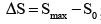
The model-free approach drives parameters directly from the signal intensity changes, including onset (lag or bolus arrival) time, maximum signal intensity, peak enhancement, time-to-peak (TTP), relative enhancement (RE), wash-in slope, wash-out slope, area under the curve (AUC) and so on (138), as shown in Figure 23.

 ,
,  relative enhancement (RE), S is the signal intensity at any time point;
  , relative peak enhancement; T0, onset (lag or bolus arrival) time, the time from contrast injection to the appearance of contrast in the tissue; Tp, time to peak (TTP), the time from the contrast injection to the signal intensity reach Smax; Tmax, Maximum acquisition time;
  , wash-in slope;
  , wash-out slope. AUC, the area under the signal intensity curve (relative).
Semi-quantitative parameters take advantage of simple definitions and easy to implement, while suffer from some limitations, including the lack of physiological meanings and variability between different scan protocol (138,139). Despite the lack of physiological interpretation, parameters derived from the model-free approach were demonstrated to be associated with the underlying physiology (140-142).
Model-based method
The model-based approach is based on pharmacokinetic models, in which the contrast concentration in liver tissues and vessels are used as basic inputs. However, DCE-MRI only acquire T1-weighted images. Thus, before modelling, a conversion from signal intensity to contrast concentration achieved by linear or nonlinear assumption is needed for both liver parenchyma and VIFs (143,144).
Nonlinear assumption
The signal intensity S(t) of a SPGR sequence is:
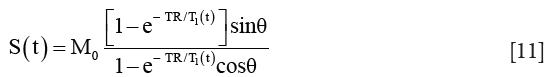
where θ is the flip angle, and M0 is the relaxed signal (TR>>T1, θ =90°), which can be calculated from the pre-contrast signal. Thus, pre-contrast T1 (T10) measurement is necessary for nonlinear conversion, which can be acquired by variable flip angle method (145) or suboptimal, assumed using published values (146).
The concentration C(t) of the contrast agents can be calculated as:
where r1 is the relaxivity, its value depends on contrast type, magnetic field strength, solvents and temperature (110).
Linear assumption
Concentration can be calculated as the relative signal intensity enhancement S(t)/S0−1, where S0 is the pre-contrast signal intensity. However, this linear assumption is just an approximation when contrast concentration is relative low, and will introduce severe bias when the contrast concentration is high, especially in AIF and PIF calculation.
Then, liver parenchyma contrast concentration and VIF can be used to fit the pharmacokinetic model. Various pharmacokinetic models have been proposed in the last few decades (Figure 24). Perfusion and liver function parameters, including arterial blood flow (Fa), portal blood flow (Fp), total hepatic blood flow (Ft), arterial fraction (ART), portal venous fraction (PV), outflow rate (Ko), distribution volume (DV), mean transit time (MTT), hepatic extraction fraction (HEF), input relative blood flow (irBF), extracellular volume (Ve), intracellular uptake rate (Ki) can be extracted from these models.

Dual input one-compartment model for extracellular agents
A dual-input one-compartment model was proposed in 2002 to quantify Fa, Fp, Ko, DV and MTT based on Gd-DOTA enhanced MRI (111). In this model, the whole liver including capillaries, extravascular spaces and cells is considered as a signal compartment (111), as shown in Figure 24A. The theoretical equation of this model is described as:

where Ct, Ca and CP represent the contrast concentration of liver parenchyma, AIF and PIF, respectively. Ta and TP represent the transit time form the aorta and portal vein to the liver. Ko is the outflow rate. ⊗ denotes the convolution operator. DV can be calculated as 100(Fa+Fp)/Ko. MTT is calculated as 1/Ko.Patients studies have demonstrated the feasibility of this model in differentiating the hepatic arterial and portal venous components in diseased liver (147-149).
Dual input two-compartment model for extracellular agents
Considering the different tracer kinetics behaviors between tumor and normal tissue, a dual input two-compartment model was proposed to assess arterial and portal blood flow, and capillary permeability in hepatic metastases (150,151). A vascular and an interstitial compartment were included for modelling liver tumors as they may develop their own vasculature (150), as shown in Figure 24B. The model is described as follow:
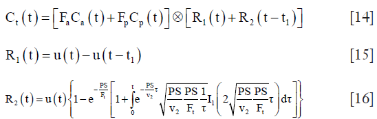
where Ct, Ca and Cp represent the contrast concentration of liver parenchyma, AIF and PIF. R1 and R2 denote the vascular transit phase and parenchyma back-flux phase. u(t) is the Heaviside unit step function. t1 is the mean time for blood to traverse the vasculature compartment. v1=Ft·t1 is the fraction vascular volume. v2 is the fraction volume of the tumor interstitial compartment. PS is the permeability-surface area product of the tumor blood vessels, and I1 is the modified Bessel function.
Deconvolution model for mixed extracellular hepatobiliary agents
For mixed extracellular hepatobiliary agents like Gd-EOB-DTPA, quantitative deconvolution method with a single blood supply was first proposed to measure HEF, which directly reflects the liver function (152-154), as shown in Figure 24C. Mathematically the response function (Ct) of the liver can be described as a convolution between the impulse response [h, also called hepatic extraction (HE) curve] and the input function (AIF, Ca):

The impulse response can be calculated using a deconvolution method. HEF and irBF are two parameters extracted from the deconvoluted HE curve. First, the hepatic retention curve (HRC) is calculated using a mono-exponential fit to several HE curve data points during hepatocyte retention phase (typically range from 420 to 1,800 s). The HRC is then extrapolated back, and HEF is defined as the ratio between the extrapolated HRC curve and the vascular peak of the HE curve. irBF is described as the initial peak value of the HE curve, which represents the blood flow in a liver ROI relative to AIF.
Dual input two-compartment model for mixed extracellular hepatobiliary agents
A dual-input two-compartment model was proposed to describe the pharmacokinetics of Gd-EOB-DTPA, which allowed a combined measurement of liver perfusion and function (reflected by intracellular uptake rate Ki) (116). Extracellular and intracellular compartments were included in this model as Gd-EOB-DTPA can be absorbed by hepatocytes (116), as shown in Figure 24D. This model is described as follow:
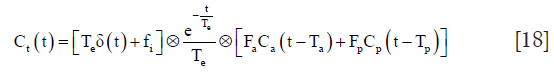
where Ct, Ca and Cp represent the contrast concentration of liver parenchyma, AIF and PIF. The extracellular mean transit time Te is calculated by Ve/(Fa+Fp+Ki). The hepatic uptake fraction fi is calculated by Ki/(Fa+Fp+Ki). Ta and Tp represent the transit time form the aorta and portal vein to the liver.
Quantitative parameters are physiologically interpretable, but they also have some technical challenges. First, the model-based approach required complex and time-consumed modelling and fitting and may result in unreliable fitting results. Second, the selection of the model is not standardized; it depends on the type of contrast agents, acquisition protocol, liver condition (healthy or diseased), pharmacokinetic assumption, and so on (117). Usually, simple models with fewer variables, such as the deconvolution model and one-compartment model, are relatively stable in model fitting and has better reproducibility, thus may be better with DCE imaging protocols with relatively low temporal resolution or low SNR. However, the simple assumption of a single blood supply or single compartment may be too simplified to reflect the real physiology of liver. On the other hand, the complex models, such as the dual input two-compartment models, are more realistic in liver physiology modelling. There are even more complex models assuming different output (venous and bile duct output) (117), but our study (117) found that complex models tend to be more unstable in model fitting while the number of model variables increase, resulting unreliable quantification. Thus, in our experience, with previously suggested widely available SPGR sequence with Cartesian trajectory (Table 1), the dual input one-compartment model proposed by Materne et al. (111) is recommended when the extracellular agents are used, while the dual-input two-compartment model proposed by Sourbron et al. (116) is recommended for mixed extracellular hepatobiliary agents analysis. Third, as discussed in the previous section, to obtain accurate VIFs is a technical challenge and may lead to fitting bias (133,136,155).
Clinical application
In liver tumors, angiogenesis is an important pathological process, different tumors have different perfusion characteristics (156-158), which can be quantified by the DCE-MRI. Thus, DCE-MRI have great potentials in classification and treatment response evolution of tumor. Taouli et al. investigated the ability of DCE-MRI for perfusion quantification of HCC and surrounding liver, they found significantly higher Fa, ART and lower DV, Fp in HCC regions compared with liver parenchyma (104). They also found higher ART, lower Fp in untreated HCCs than chemoembolized HCCs (104).
Quantitative parameters derived from DCE-MRI have also been investigated to monitor the treatment response of tumors to antiangiogenic drugs. Morgan et al. assessed tumor permeability and vascularity by calculating the bidirectional transfer constant using DCE-MRI in advanced colorectal cancer and liver metastases patients who received PTK787/ZK 222584 therapy (105). Their results showed patients with a best response of stable disease had a significantly greater reduction in bidirectional transfer constant at both day 2 and at the end of cycle 1 (28-day) compared with progressors, and demonstrated that DCE-MRI may be a useful biomarker for the pharmacological response of angiogenesis inhibitors (105). Wang et al. used DCE-MRI to evaluate the perfusion changes in advanced HCC patients who were treated with the antiangiogenic agent thalidomide (106). Significant differences were found for the semiquantitative parameters including the peak enhancement, the maximal enhancement, and the enhancement slope percentage between patients who had progressive disease and who had stable disease or partial response (106).
In recent years, the potential of DCE-MRI with mixed extracellular hepatobiliary agents has drawn more and more interests from researchers in the prediction of post-operative (partial liver resection for tumor treatment) liver failure. In this unique application, instead of quantifying the perfusion characteristics of tumor, the major aim is to quantify the remnant liver function by quantifying the uptake or the uptake rate of mixed extracellular hepatobiliary agents into hepatocytes (109).
The challenge and future of DCE-MRI
Although DCE-MRI can provide physiological meaningful and quantitative perfusion characteristics, its low reliability is still the biggest challenge for its use in clinical practice. Aronhime et al. reported a range of 11.87–73.16% of the interscan reproducibility for the perfusion parameters in patients with chronic hepatitis (144). The low reliability can be caused by its motion artifacts, image blurring and the uncertainty of pharmacokinetic analysis. Also, considering the relatively low spatial resolution and poor image quality of liver DCE images, and its potential conflict in the imaging protocol arrangement with traditional multi-phase contrast-enhanced MRI, which has higher spatial resolution and image quality, DCE-MRI has not become the mainstream technology in clinical practice till now. Thus, improving the spatial resolution, image quality and the quantification reliability using advanced MR imaging and reconstruction techniques should be the keys to translate liver DCE-MRI into clinical practice. Improvement of liver DCE-MRI technique to achieve comparable performance with current multi-phase contrast-enhanced MRI in the aspects of reliability, spatial resolution and image quality should be the major goal of technical development.
Liver fat quantification
NAFLD, excessive triglycerides (TG) accumulated in the liver, is associated with increased metabolic risk factors such as obesity, diabetes mellitus, and dyslipidemia. This fatty liver disease is an increasing health issue in the global population, with prevalence ranges from 9% to 37% worldwide (159-164). However, since TG accumulation is potentially reversible, fat quantification for diagnosis of NAFLD at an early stage in the liver helps to introduce lifestyle modifications and pharmacological therapies to prevent progression of the disease.
Liver fat quantification by biopsy suffers from the sampling variability to obtain a representation of the whole liver (165,166), and this semi-quantitative grading of hepatic steatosis is strongly observer-dependent (167,168). There has been ultrasonography (US) technique developed to screen subjects at risk of NAFLD. However, it may not be ideal for detecting mild steatosis or monitoring NAFLD patients after therapeutic interventions because of its operator dependency and its qualitative nature in the absence of dedicated image post-processing (169).
Magnetic resonance spectroscopy (MRS)
In vivo proton MRS (1H-MRS) provides a noninvasive means of liver fat content quantification (170). Stimulated Echo Acquisition Mode (STEAM) sequence is usually applied to acquire MRS signal (171), which allows the shortest minimum echo time (TE) and the mixing time (TM) to minimize J-coupling effects (172). A long TR (>3,000 ms) is used to minimize T1 effects. Multiple STEAM spectra (≥5) with various TEs are acquired consecutively in a single acquisition to estimate the T2 of water and fat peaks, which is further used to correct the T2 effect (Figure 25). It has been acknowledged as an accurate and the most sensitive noninvasive method to assess hepatic steatosis with clinically accepted sensitivity and has been used as the reference standard in several clinical studies to determine the prevalence of hepatic lipid content in the general adult population (173-175). However, MRS is not routinely used for the reason that it is time-consuming and requires user expertise to perform and analyze spectroscopy data (176); in addition, the limitation of spatial coverage and prone to liver inhomogeneity restrain its application for a clinical routine examination.

Chemical shift encoded MRI (CSE-MRI)
The CSE-MRI technique can discriminate between fat and water spins based on their different resonance frequencies. The quantitative proton density fat fraction (PDFF) has been proposed and studied well as a quantitative MRI method which covers large parts of the liver or the entire organ without the use of contrast agents (9,10,177,178). It was developed based on the DIXON method in utilizing the periodic change in MR signal because of the hydrogen Larmor frequency difference in water and fat (8). The 2-echo method with in-phase (when water and lipid signals align in the same direction) and out-of-phase measurements (when water and lipid hydrogen move to the opposite directions) was initially evaluated for the feasibility of hepatic fat fraction measurement, but its clinical applications still restrict to obtain the qualitative imaging such as the water-only (or fat-suppressed) or fat-only images. The 6-echo DIXON method has proven an advantage in quantifying fat content comparing to 2-echo method (179). To accomplish multi-echo scan in one breath-hold, and to restrict the long echo time, modified DIXON (mDIXON) technique is used to permit flexible echo time (TE) instead of exact in-phase/out-of-phase TE. B0 inhomogeneity needs to be corrected to best utilize acquired MRI signal at each echo time. A small flip angle is used to minimize T1 bias (180,181). Table 2 shows an example of PDFF protocol with 6 evenly distributed echoes, and this sequence lasts 15.5 s.

Full table
T2* decay needs to be addressed in the multi-echo MR signal model to compensate additional MR signal change from the 1st echo to the last one. A 20-echo gradient-echo MRI method for PDFF in rats finds a strong correlation with biochemical measurements of the fat content fraction (182). In their study, the T2* difference of water and lipid was taken into consideration in signal modelling because the echo train is long. A later study in measuring fat content in geese livers demonstrated that PDFF value generated by a 6-echo CSI-MR method was almost equivalent to fat fraction measured by biochemical TG content extraction (183). The improvement would be attributed to the inclusion of the multi-peak spectral model for fat quantification calculation, as MRS identifies several lipid components corresponding to different chemical groups in fatty acids chain. The multi-peak spectral model (184) usually has been correlated with 1H-MRS and histological findings (185,186). Table 3 lists the percentage of signal contribution by each peak, provided by the 7-peak lipid model in Philips Ingenia MRI units, accounting for 10 TG components to calculate PDFF values with the mDIXON Quant sequence. The signal ratio of the (CH2)n component from the bulk methylene protons as determined by MRS 62.5% with a slight variation of 1.2% depending on the type of TG structure.

Full table
The multi-echo CSE-MRI technique incorporating multi-peak spectral model can be summarized as the equation below, with the corrections for T2* decay:
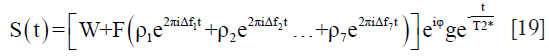
where S(t) is the signal acquired at different echo times (t = TE1, TE2, TE3 and more); W and F are the amplitudes of water and fat signals; ρi stands for the ratio of each peak in the multi-peak lipid MR signal model, with Δfi corresponding to each Larmor frequency with respect to water proton frequency. T2* is introduced to compensate signal decay during the multi-echo train, and the phase φ measured at each echo is used to compensate B0 inhomogeneity. Then, a nonlinear fitting algorithm can be used to derive solutions of W, F and T2*. Consequently, the PDFF is calculated as:
Multi-echo CSE-MRI has been validated with excellent correlation with MRS and histological methods for quantification of fat content (11,183,186). Figure 26 shows a direct output of water, fat only images, fat fraction maps and T2* maps.

This CSE-MRI method can be influenced by many factors, including noise bias (180), the lipid spectral complexity and eddy currents (181,185). The CSE-MRI results can also deviate from fat quantitation by chemical extraction method because PDFF is the ratio of lipid MR signal fraction in all protons while biochemical extraction measures the TG content weight fraction in the liver. In addition, CSE-MRI cannot measure protons with very short T2* such as hydrogen protons closely connected to large proteins or contents other than protons, which further compromise the equivalence of PDFF and fat weight density fraction. The different T2* decay (181,185) of water and lipids (typically around 23 and 45 ms in liver in a 3T scanner, respectively) need also to be accounted for in the different CSE-MRI methods with very long echo train to determine PDFF (182), though it has been demonstrated that single-T2* model performs best for short TEs over a range of clinically relevant signal-to-noise ratios (SNRs) and water/fat ratios (187). These factors generate systematic shifts in the hepatic fat fraction values and may explain the difference with results obtained by biochemical extraction (183). With these confounding factors impacting accuracy of PDFF, CSE-MRI result is complicated, hence filters are applied in the PDFF in clinical use for liver fat quantification to gain stability and get rid of irrelevant influences.
Liver iron quantification (LIC)
Measurement of LIC is critical for assessing the magnitude of the body iron burden in the diagnosis and management of both hereditary and acquired forms of iron overload (188). MRI is highly sensitive to paramagnetic iron and has emerged as the primary non-invasive modality for tissue iron quantification in evaluating iron overload and monitoring iron-chelating therapy (189).
Liver iron, typically present in the form of paramagnetic ferritin or hemosiderin, increases the susceptibility of tissue and creates a local susceptibility-induced contribution to the local magnetic field. Liver iron has an influence on the relaxation times of the liver parenchyma, most notably T2 and T2*. T2 represents the time constant of the intrinsic decay of the transverse magnetization from spin-spin interactions, while T2* also incorporates effects from local magnetic field inhomogeneities:
where T2' is the additional contribution from field inhomogeneities. T2 and T2* can also be represented as relaxation rates, such that:
T2 and T2* will be shortened (i.e., the relaxation rates R2 and R2* will be increased) with an increase in the iron concentration (190-192) (Figure 27), resulting in the decreased signal intensity on T2- and T2*-weighted images (Figure 28). Several quantitative MR-based strategies have been employed to measure LIC: signal intensity ratio (SIR) techniques based on T2-weighted or T2*-weighted imaging, quantitative relaxometry (largely R2- and R2*-based), and MR quantitative susceptibility mapping (QSM) (Figure 28).


SIR techniques
In SIR methods, the signal intensity of the liver on spin-echo or GRE sequences is divided by the signal intensity of a reference tissue that does not accumulate iron, such as paraspinal muscles (193-195). The body coil is used as the receive coil to achieve homogeneous signal intensity in the imaged section and avoid spatial sensitivity variations arising from phased-array coils (196,197). The use of an MR scanner with a B1 correction method or dielectric cushion is recommended to avoid an artificial decrease in paraspinal muscle signal intensity (197).
The most widely used SIR method is the one established by Gandon’s group (195-197). Five images, one proton density image with a minimal opposed-phase TE and four T2*-weighted images with varying in-phase TEs, are obtained with a breath-hold multi-echo GRE sequence (196) or five breath-hold single-echo GRE sequences (195,197). The long TR (i.e., 120 ms) and low flip angle (i.e., 20°) are used to remove the T1-weighting effect. Liver and muscle signal intensity measurements are performed on three ROIs within the right lobe of the liver, and in two ROIs in the right and left paraspinal muscles, respectively (Figure 29). Thus, each of the five images results in a different liver/muscle signal intensity ratio. These five values are then combined to provide a LIC estimate using a specialized algorithm (195). The acquisition protocols and calculations are provided online for MR imaging field strengths of 1T, 1.5T, and 3T (www.mrquantif.org).

The SIR method is easy to implement and inexpensive; it represents a viable alternative for screening in a clinical setting, particularly for centers without relaxometry methods (198). However, this technique is not accurate for severe iron overload exceeding 350 µmol/g dry weight (19.5 mg/g dry weight) and tends to overestimate mild and moderate liver iron overload. Further, the technique is dependent on the assumption that the reference tissue is normal. While paraspinal muscles may not be affected by iron overload, muscle atrophy and fat infiltration, especially in elderly patients, may confound the T2* of the muscles (195,197). Moreover, it is unclear how factors such as liver steatosis affect SIR measurements (189), while confounding factors such as fat can be corrected in R2* Relaxometry.
R2 relaxometry
R2 can be estimated from a series of spin-echo signals acquired at various echo times by modelling the decay of the spin-echo signal magnitude with TE as a mono-exponential or bi-exponential (191,199,200). With the background signal level and mono-exponential model taken into consideration, the decay in signal intensity following the spin-echo pulse sequence is given by:

where S(TE) is the magnitude of signal intensity at TE, S0 is the initial magnitude of signal intensity at TE=0 ms, and B is a constant term that takes into account the fact that noise prevents the signal to decay to zero in long TE sequences. This equation is fitted to the voxel intensity data as a function of TE.
St Pierre et al. derived an empirical curvilinear expression for R2 in terms of LIC (Figure 27) and validated the calibration curve in a multicenter study (201). In their method, axial images are acquired with a multislice single echo SE pulse sequence, with a pulse repetition time of 2,500 ms, TEs of 6, 9, 12, 15, and 18 ms, and slice thickness of 5 mm. A 1,000 mL bag of normal saline solution is placed in the FOV and imaged with each patient to provide an external long T2 reference for the correction of instrumental gain drift and signal intensity variations due to any bandwidth changes. Typical data acquisition time is 22 min. R2 is calculated by fitting the image signal intensities measured at each TE with bi-exponential model after corrections for signal gain drift, noise bias, and radiofrequency field inhomogeneities are performed. The liver iron content is estimated by using the calibration curve.
An important advantage of the St Pierre method is that it has received Food and Drug Administration (FDA) approval, and is commercially available as FerriScan, provided by Resonance Health Inc (https://www.resonancehealth.com/). A multicenter study indicated that the calibration curve for FerriScan is independent of scanner type, stage of liver fibrosis, the grade of necroinflammation (201). However, upper and lower 95% limits of agreement between R2-MRI and biopsy LIC measurements were 74% and −71% (201). These errors in liver iron estimation can be problematic in clinical practice. Additionally, R2 mapping requires a long scanning time, which causes potentially severe motion artifacts in free-breathing acquisitions. It also requires additional cost and delay for the data analysis.
R2* relaxometry
R2* relaxometry based on multi-echo gradient-echo acquisitions can provide full liver coverage without motion artifacts within a single breath-hold (189). R2* values are calculated by fitting an exponential model to the GRE datasets with various TEs. However, conventional R2* mapping is affected by two key confounding factors: noise-related bias and the presence of fat in tissue.
The Rician-distributed noisy magnitude data cause a ‘‘noise floor’’ with nonzero mean at low SNR, which leads to an underestimation of R2* in cases with low SNR or the presence of very rapid R2* decay (Figure 30A). The truncation (202), baseline fitting (203), the first and second-moment noise corrected models (204), and complex fitting (205) have been used to address the noise-related bias. The bias can partially be corrected with noise floor fitting techniques, which attempt to model the noise floor by adding a constant to the signal model (Figure 30B). Truncation techniques remove the later echoes with low signal intensity and then the remaining echoes are fitted with a mono-exponential equation (Figure 30C). Complex fitting avoids noise bias because the Gaussian zero-mean noise is preserved (Figure 30D). Ultrashort TE techniques based on radial acquisitions have been proposed to extend the dynamic range of R2* relaxometry techniques for cases of low SNR with massive iron overload (206-208).

In the presence of water and fat signal components, the signal acquired at a single voxel is not a simple mono-exponential decay, but instead contains oscillations (Figure 31). One simple approach to address the effects of fat in R2* mapping is to acquire images at TEs where the water and main methylene resonance of fat (217 and 434 Hz from water peak at 1.5T and 3T, respectively) are “in-phase” (4.6 ms, 9.2 ms, etc., at 1.5T; 2.3 ms, 4.6 ms, etc., at 3T) (210). However, this approach does not account for the spectral complexity of the fat signal and do not permit accurate R2* estimation (205) (Figure 31). Moreover, in-phase echoes may be too long to capture the signal decaying in heavy iron overload.

The most popular fat-corrected R2* measurement is a chemical shift-based R2* estimation method with multiple peaks fat modelling (205,209,211,212). In the presence of water and fat signal components, the signal acquired at a single voxel can be modelled by the following signal equation:
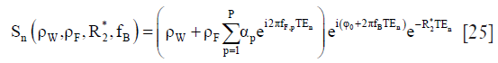
where ρW and ρF are the amplitudes of water and fat signals, respectively, with the initial phase φ0, R2* =1/T2*, fB is the frequency shift due to local magnetic field inhomogeneities, fF,p are the known frequencies for the multiple spectral peaks of the fat signal relative to the water peak, αp are the relative amplitudes of the fat signal. Fat-corrected R2* measurements can be obtained by jointly performing fat-water separation and R2* estimation.
In multiple studies, R2* has been demonstrated to have a linear correlation with biopsy-determined liver iron content and calibrations for converting R2* into LIC have been investigated (192,213,214), which demonstrated R2* relaxometry is a reliable technique for noninvasive liver iron overload quantification (215). However, the calibration curves depend on acquisition protocols, postprocessing models and different biopsy-LIC measurements (192,213,214,216,217). The R2* at 3.0 T is twice that at 1.5T (189,218-220). Thus the empirical calibration curves are validated only for the particular field strength, imaging parameters, and reconstruction technique.
MR QSM
While the magnitude data of the multi-echo gradient-echo is used to generate R2*, the phase data can be used to generate quantitative susceptibility maps to directly measure magnetic susceptibility (221,222) without blooming artifacts found in R2* (223). QSM has been applied to abdominal organs by accounting for the fat contribution to the measured signal phase (219,224-226).
In MRI, the tissue local magnetic field can be approximated as the convolution of the dipole kernel with the susceptibility distribution (227):
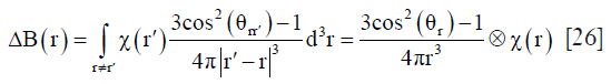
where ΔB(r) is the local field measured relative to B0, 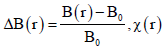 is the spatially varying susceptibility distribution, r and r′ refer to the locations of the observed field and susceptibility source, respectively, θr is the azimuthal angle of r in the spherical coordinate (The subscript r is typically omitted).
The pulse sequence for liver QSM is a 3D breath-hold multi-echo GRE, which is same as that for R2* mapping. After performing fat-water separation and R2* estimation based on Eq. [25], magnetic field inhomogeneities are also estimated. However, the measured field inhomogeneities include local magnetic field generated by the human body itself and the background field contributed by sources outside a ROI. The background field can be removed with the assumption that the phase created inside the ROI by outside sources is harmonic. After background field removal, the susceptibility map is then estimated using the dipole inversion technique based on Eq. [26]. Figure 32 shows the typical processing pipeline to estimate the susceptibility maps in the abdomen.

Magnetic susceptibility is an intrinsic tissue property linearly related to liver iron (219,226,228,229). QSM is potentially the most direct and most sensitive MR imaging technique for detection of iron deposition. Liver susceptibility estimates demonstrate good correlation with both Ferriscan-LIC (R2=0.76 at 1.5T, R2=0.83 at 3T) and liver R2* (R2=0.94 at 1.5T, R2=0.93 at 3T) (219). However, QSM is not sensitive to the cases with extremely high LIC, due to iron-related low SNR (228,230). To generate QSM with massive liver iron overload, ultrashort echo time (UTE) sequences may be used to acquire sufficient signal in patients with very rapid T2* signal decay (231). Another limitation of QSM is that the exact relationship between QSM values and liver iron content is not yet clearly established.
Scan speed acceleration and movement reduction techniques
The introduction of multichannel, multi-element phased array coils allows parallel imaging techniques by accelerating the k-space acquisition to reduce scan time and related artefacts such as susceptibility artefacts, and dramatically improved SNR. Acceleration factors are typically limited by the inducement of residual artefacts and signal loss. Acronyms of parallel imaging techniques include GeneRalized Autocalibrating Partially Parallel Acquisitions (GRAPPA) (121), SENSitivity Encoding (SENSE) (120), Array coil Spatial Sensitivity Encoding (ASSET) and sequence integrated with automated coil calibration (mSENSE). ‘Low–high’ is a commonly used k-space filling order in liver breath-hold imaging, that the central part of the k-space is acquired at first when the patient can hold breath well while the outer part of the k-space is acquired later when unintentional tremor may present, and thus reduce motion artefacts. Sampling trajectories like radial, spiral and Periodically Rotated Overlapping ParallEL Lines with Enhanced Reconstruction (PROPELLER) (232) oversample the k-space center region (Figure 33), granting these methods intrinsic immunity to motion artefacts. By using advanced post-processing techniques to registrate each line or blade based on this oversampled k-space center for image reconstruction, the motion artefacts could be further reduced to a lower level (232,233). The drawback of radial and PROPELLER acquisition is the prolonged acquisition time compared with a traditional Cartesian acquisition.

Other fast imaging strategies can also be used in liver imaging to reduce respiratory motion artefacts. Fast sequences like turbo field echo (TFE) (234), balanced steady-state free precession (bSSFP) (235), single-shot turbo spin echo (TSE) (236) and echo planar imaging (EPI) are widely used in liver imaging (237). In the meantime, fast imaging method like SENSE, GRAPPA, compressed sensing (CS) (122), half scan, partial echo techniques can also be combined with these fast imaging sequences to further reduce total scan time. To acquire all slices in a single breath-hold, several fast imaging methods like SENSE, GRAPPA, CS and half scan, which omit k-space samples, can be used. However, those k-space sampling reduction techniques lead to SNR decrease in most cases for conventional imaging applications, even though the SNR penalty for DW-MR imaging can be mitigated due to decreased echo time. At the meantime, these fast imaging methods can increase the bandwidth of echo planar imaging (EPI), therefore reduce the geometry distortion (238).
DW-MRI or diffusion tensor imaging (DTI) acquires multi-slice data with multiple diffusion directions and multiple number-of-signal-averaging (NSAs), hence its total scan time would be prolonged. To accelerate the acquisition speed, simultaneous multi-slice (SMS) with blipped CAIPIRINHA (controlled aliasing in parallel imaging results in higher acceleration) (239-241) can be used. This simultaneous acquisition technique will not lead to an  decrease on SNR (R represents acceleration factor) (239), compared with traditional parallel imaging methods with arrayed receiving coils. This SMS method has been mostly implemented in the brain, while studies demonstrated its feasibility in abdominal use such as liver imaging.
To catch the signal intensity changes after applying the contrast agent, high imaging speed is needed. Unlike the aforementioned fast imaging methods, which make use of spatial correlation, techniques utilize temporal correlations, such as keyhole (123,124) and view sharing (125,242), are also commonly used by commercial scanners (Figure 34). These techniques can accelerate dynamic imaging by sharing peripheral k-space data because the image contrast is mainly determined by the central k-space data. Other useful techniques which utilize both temporal and spatial correlations, like k-t BLAST/k-t SENSE (127) and k-t GRAPPA (128) are developed to achieve even higher acceleration. These methods are based on that dynamic images exhibit significant signal correlations in k-space and time, which can be learned from a small set of training data (127) or locally derived from the acquired data (128), then the missing data can be recovered. In 2014, a novel technique named iGRASP (iterative Golden-angle RAdial Sparse Parallel MRI) (243) was proposed to combine CS, parallel imaging and golden-angle radial sampling strategies together, which in our experience, performs well and provides a promising fast free-breathing dynamic volumetric MRI technique with high spatial-temporal resolution.

To overcome the challenging groups of the elderly or pediatric patients with poor breath-hold capacity, in-plane radial sampling using a fat-suppressed spoiled-GRE T1 weighted sequence (Siemens: Star VIBE; Philips: 3D VANE XD) has been explored and introduced for clinical use. This method shows good motion robustness and advantage in free-breathing imaging (244).
MRI provides a multi-contrast and multi-parametric modality to diagnosis and evaluate liver diseases. This article only covers selected topic on liver quantitative MRI, and a number of highly relevant technologies are not included. MR Elastography assesses tissue stiffness by measuring the speed of shear waves propagating within it. With the addition of a special hardware (i.e., driver), MR elastography has been used for diagnosing and staging liver fibrosis with very promising results. However, detection of stage-1 liver fibrosis remain challenging using MR Elastography (48). T1rho has been shown to be promising in assessing liver inflammation and collagen deposition, i.e., factors associated with fibrosis (245,246), though the underlying mechanism for T1rho elevation in liver fibrosis has not been fully explained (247). The work of Xie et al. (248) suggests T1rho may differentiate simple steatosis from liver pathologies involving inflammation and fibrosis such as NASH. In a study of rabbit model, Xie et al. (249) reported T1rho imaging during the hepatobiliary phase of Gd-EOB-DTP allowed a total separation of normal livers and livers with NASH [Figure 2B of (249)], such a differentiation was better than T1rho alone [Figure 2A of (249)]. On the other hand, it has been noted that liver T1rho in healthy subjects is age and gender dependent, and female subjects and younger subjects have higher T1rho measures (78). In investigative studies, it can often be the case that liver fibrosis subjects (elevated liver T1rho) are older than controls (younger subjects have higher liver T1rho), and the difference between cirrhosis subjects and controls may be ‘artificially’ reduced. Therefore, for comparative studies, controls should be age- and gender-matched. Measurement correction methods for liver iron deposition are also expected to be useful (247). T1 mapping [using Lock-Lock, modified Look-Locker inversion recovery (MOLLI), shortened Modified Look-Locker Inversion recovery (ShMOLLI)] before and after Gd have been investigated in evaluating different kind of liver diseases and liver functions (175,250). 3D acquisition methods are also being investigated using dual or multi-flip angles sequences for T1 mapping. Recently, the interest of a SPIO (superparamagnetic iron oxide) type of contrast agent Ferumoxytol (Feraheme; AMAG Pharmaceuticals, USA) has been re-ignited (251,252). Ferumoxytol is approved in the United States and Europe for use in the intravenous treatment of iron deficiency anemia, it can be used as an injectable bolus blood pool contrast agent for MRI. With the recent confirmation of its safety profile (252,253), it is expected this SPIO type of contrast agent may find its application in liver imaging. Furthermore, various algorithms of artificial intelligence are being developed very rapidly that may play an important role in the detection, segmentation, and classification of liver diseases. Future development directions also include standardization of the quantification methods through multi-centre validation, as well as continuous improvement of the temporal and spatial resolution, making liver imaging faster and more robust against physiological motions.
Acknowledgments
Author YX Wang thanks Dr Olivier Chevallier, former research fellow at the Chinese University of Hong Kong and currently staff Radiologist with François-Mitterrand University Hospital, Dijon Cedex, France; Dr Hua Huang, staff Radiologist at the Third People’s Hospital of Shenzhen, Shenzhen, China; and Mr Nazmi Che-Nordin, research student at the Chinese University of Hong Kong, for their contributions to the IVIM part of this paper. Dr Weitian Chen helped the examination setup for single breathhold IVIM data acquisition.
Footnote
Weibo Chen was the coordinator of this paper. Yi-Xiang Wang was primarily responsible for the writing-up of sections of DW-MR Imaging and IVIM; Xiaoqi Wang was primarily responsible for the writing-up of sections of fat signal suppression and liver fat quantification; Peng Wu was primarily responsible for the writing-up of section of fast data acquisition; Huijun Chen was primarily responsible for the writing-up of section of DCE-MRI; Jianqi Li was primarily responsible for the writing-up of section of liver iron quantification. All authors approved the content of this paper.
Conflicts of Interest: Xiaoqi Wang, Peng Wu, and Weibo Chen are employees of Philips Healthcare.
References
- Delfaut EM, Beltran J, Johnson G, Rousseau J, Marchandise X, Cotten A. Fat suppression in MR imaging: techniques and pitfalls. Radiographics 1999;19:373-82. [Crossref] [PubMed]
- Morrell GR. Rapid fat suppression in MRI of the breast with short binomial pulses. J Magn Reson Imaging 2006;24:1172-6. [Crossref] [PubMed]
- Del Grande F, Santini F, Herzka DA, Aro MR, Dean CW, Gold GE, Carrino JA. Fat-suppression techniques for 3-T MR imaging of the musculoskeletal system. Radiographics 2014;34:217-33. [Crossref] [PubMed]
- Bley TA, Wieben O, Francois CJ, Brittain JH, Reeder SB. Fat and water magnetic resonance imaging. J Magn Reson Imaging 2010;31:4-18. [Crossref] [PubMed]
- Forrai G, Polgar C, Zana K, Riedl E, Fodor J, Nemeth G, Fornet B. The role of STIR MRI sequence in the evaluation of the breast following conservative surgery and radiotherapy. Neoplasma 2001;48:7-11. [PubMed]
- Dietrich TJ, Ulbrich EJ, Zanetti M, Fucentese SF, Pfirrmann CW. PROPELLER technique to improve image quality of MRI of the shoulder. AJR Am J Roentgenol 2011;197:W1093-100. [Crossref] [PubMed]
- Kato H, Kuroda M, Yoshimura K, Yoshida A, Hanamoto K, Kawasaki S, Shibuya K, Kanazawa S. Composition of MRI phantom equivalent to human tissues. Med Phys 2005;32:3199-208. [Crossref] [PubMed]
- Dixon WT. Simple proton spectroscopic imaging. Radiology 1984;153:189-94. [Crossref] [PubMed]
- Berglund J, Ahlstrom H, Johansson L, Kullberg J. Two-point dixon method with flexible echo times. Magn Reson Med 2011;65:994-1004. [Crossref] [PubMed]
- Eggers H, Brendel B, Duijndam A, Herigault G. Dual-echo Dixon imaging with flexible choice of echo times. Magn Reson Med 2011;65:96-107. [Crossref] [PubMed]
- Noble JJ, Keevil SF, Totman J, Charles-Edwards GD. In vitro and in vivo comparison of two-, three- and four-point Dixon techniques for clinical intramuscular fat quantification at 3 T. Br J Radiol 2014;87:20130761. [Crossref] [PubMed]
- Kim SW, Kim CH, Kim MS, Jung YJ, Byun WM. Usefulness of Three Dimensional Proset MR Images for Diagnosis of Symptomatic L5-S1 Foraminal and Extraforaminal Stenosis. J Korean Neurosurg Soc 2013;54:30-3. [Crossref] [PubMed]
- Hauger O, Dumont E, Chateil JF, Moinard M, Diard F. Water excitation as an alternative to fat saturation in MR imaging: preliminary results in musculoskeletal imaging. Radiology 2002;224:657-63. [Crossref] [PubMed]
- Le Bihan D, Breton E, Lallemand D, Grenier P, Cabanis E, Laval-Jeantet M. MR imaging of intravoxel incoherent motions: application to diffusion and perfusion in neurologic disorders. Radiology 1986;161:401-7. [Crossref] [PubMed]
- Le Bihan D, Turner R, Moonen CT, Pekar J. Imaging of diffusion and microcirculation with gradient sensitization: design, strategy, and significance. J Magn Reson Imaging 1991;1:7-28. [Crossref] [PubMed]
- Winston GP. The physical and biological basis of quantitative parameters derived from diffusion MRI. Quant Imaging Med Surg 2012;2:254-65. [PubMed]
- Stejskal EO, Tanner JE. Spin diffusion measurements: spin echoes in the presence of a time-dependent field gradient. The journal of chemical physics 1965;42:288-92. [Crossref]
- Norris DG. The effects of microscopic tissue parameters on the diffusion weighted magnetic resonance imaging experiment. NMR Biomed 2001;14:77-93. [Crossref] [PubMed]
- Mürtz P, Flacke S, Traber F, van den Brink JS, Gieseke J, Schild HH. Abdomen: diffusion-weighted MR imaging with pulse-triggered single-shot sequences. Radiology 2002;224:258-64. [Crossref] [PubMed]
- Butts K, Riederer SJ, Ehman RL, Felmlee JP, Grimm RC. Echo-planar imaging of the liver with a standard MR imaging system. Radiology 1993;189:259-64. [Crossref] [PubMed]
- Turner R, Le Bihan D, Chesnick AS. Echo-planar imaging of diffusion and perfusion. Magn Reson Med 1991;19:247-53. [Crossref] [PubMed]
- Bammer R. Basic principles of diffusion-weighted imaging. Eur J Radiol 2003;45:169-84. [Crossref] [PubMed]
- Koh DM, Collins DJ. Diffusion-weighted MRI in the body: applications and challenges in oncology. AJR Am J Roentgenol 2007;188:1622-35. [Crossref] [PubMed]
- Padhani AR, Liu G, Koh DM, Chenevert TL, Thoeny HC, Takahara T, Dzik-Jurasz A, Ross BD, Van Cauteren M, Collins D, Hammoud DA, Rustin GJ, Taouli B, Choyke PL. Diffusion-weighted magnetic resonance imaging as a cancer biomarker: consensus and recommendations. Neoplasia 2009;11:102-25. [Crossref] [PubMed]
- Guiu B, Cercueil JP. Liver diffusion-weighted MR imaging: the tower of Babel? Eur Radiol 2011;21:463-7. [Crossref] [PubMed]
- Bülow R, Mensel B, Meffert P, Hernando D, Evert M, Kühn JP. Diffusion-weighted magnetic resonance imaging for staging liver fibrosis is less reliable in the presence of fat and iron. Eur Radiol 2013;23:1281-7. [Crossref] [PubMed]
- Taouli B, Koh DM. Diffusion-weighted MR imaging of the liver. Radiology 2010;254:47-66. [Crossref] [PubMed]
- Shenoy-Bhangle A, Baliyan V, Kordbacheh H, Guimaraes AR, Kambadakone A. Diffusion weighted magnetic resonance imaging of liver: Principles, clinical applications and recent updates. World J Hepatol 2017;9:1081. [Crossref] [PubMed]
- Chandarana H, Taouli B. Diffusion-weighted MRI and liver metastases. Magn Reson Imaging Clin N Am 2010;18:451-64. x. [Crossref] [PubMed]
- Piana G, Trinquart L, Meskine N, Barrau V, Beers BV, Vilgrain V. New MR imaging criteria with a diffusion-weighted sequence for the diagnosis of hepatocellular carcinoma in chronic liver diseases. J Hepatol 2011;55:126-32. [Crossref] [PubMed]
- Vandecaveye V, De Keyzer F, Verslype C, De Beeck KO, Komuta M, Topal B, Roebben I, Bielen D, Roskams T, Nevens F. Diffusion-weighted MRI provides additional value to conventional dynamic contrast-enhanced MRI for detection of hepatocellular carcinoma. Eur Radiol 2009;19:2456-66. [Crossref] [PubMed]
- Parikh T, Drew SJ, Lee VS, Wong S, Hecht EM, Babb JS, Taouli B. Focal liver lesion detection and characterization with diffusion-weighted MR imaging: comparison with standard breath-hold T2-weighted imaging. Radiology 2008;246:812-22. [Crossref] [PubMed]
- Tang Y, Wang H, Ma L, Zhang X, Yu G, Li J, Ye H. Diffusion-weighted imaging of hepatocellular carcinomas: a retrospective analysis of correlation between apparent diffusion coefficients and histological grade. Abdom Radiol (NY) 2016;41:1539-45. [Crossref] [PubMed]
- Okamura S, Sumie S, Tonan T, Nakano M, Satani M, Shimose S, Shirono T, Iwamoto H, Aino H, Niizeki T, Tajiri N, Kuromatsu R, Okuda K, Nakashima O, Torimura T. Diffusion-weighted magnetic resonance imaging predicts malignant potential in small hepatocellular carcinoma. Dig Liver Dis 2016;48:945-52. [Crossref] [PubMed]
- Nakanishi M, Chuma M, Hige S, Omatsu T, Yokoo H, Nakanishi K, Kamiyama T, Kubota K, Haga H, Matsuno Y, Onodera Y, Kato M, Asaka M. Relationship between diffusion-weighted magnetic resonance imaging and histological tumor grading of hepatocellular carcinoma. Ann Surg Oncol 2012;19:1302-9. [Crossref] [PubMed]
- Heo SH, Jeong YY, Shin SS, Kim JW, Lim HS, Lee JH, Koh YS, Cho CK, Kang HK. Apparent diffusion coefficient value of diffusion-weighted imaging for hepatocellular carcinoma: correlation with the histologic differentiation and the expression of vascular endothelial growth factor. Korean J Radiol 2010;11:295-303. [Crossref] [PubMed]
- Nishie A, Tajima T, Asayama Y, Ishigami K, Kakihara D, Nakayama T, Takayama Y, Okamoto D, Fujita N, Taketomi A, Yoshimitsu K, Honda H. Diagnostic performance of apparent diffusion coefficient for predicting histological grade of hepatocellular carcinoma. Eur J Radiol 2011;80:e29-33. [Crossref] [PubMed]
- Catalano OA, Choy G, Zhu A, Hahn PF, Sahani DV. Differentiation of malignant thrombus from bland thrombus of the portal vein in patients with hepatocellular carcinoma: application of diffusion-weighted MR imaging. Radiology 2010;254:154-62. [Crossref] [PubMed]
- Koh DM, Scurr E, Collins D, Kanber B, Norman A, Leach MO, Husband JE. Predicting response of colorectal hepatic metastasis: value of pretreatment apparent diffusion coefficients. AJR Am J Roentgenol 2007;188:1001-8. [Crossref] [PubMed]
- Schraml C, Schwenzer NF, Martirosian P, Bitzer M, Lauer U, Claussen CD, Horger M. Diffusion-weighted MRI of advanced hepatocellular carcinoma during sorafenib treatment: initial results. AJR Am J Roentgenol 2009;193:W301-7. [Crossref] [PubMed]
- Tam HH, Collins DJ, Brown G, Chau I, Cunningham D, Leach MO, Koh DM. The role of pre-treatment diffusion-weighted MRI in predicting long-term outcome of colorectal liver metastasis. Br J Radiol 2013;86:20130281. [Crossref] [PubMed]
- Anzidei M, Napoli A, Zaccagna F, Cartocci G, Saba L, Menichini G, Cavallo Marincola B, Marotta E, Di Mare L, Catalano C, Passariello R. Liver metastases from colorectal cancer treated with conventional and antiangiogenetic chemotherapy: evaluation with liver computed tomography perfusion and magnetic resonance diffusion-weighted imaging. J Comput Assist Tomogr 2011;35:690-6. [Crossref] [PubMed]
- Cui Y, Zhang XP, Sun YS, Tang L, Shen L. Apparent diffusion coefficient: potential imaging biomarker for prediction and early detection of response to chemotherapy in hepatic metastases. Radiology 2008;248:894-900. [Crossref] [PubMed]
- Thoeny HC, De Keyzer F, Vandecaveye V, Chen F, Sun X, Bosmans H, Hermans R, Verbeken EK, Boesch C, Marchal G, Landuyt W, Ni Y. Effect of vascular targeting agent in rat tumor model: dynamic contrast-enhanced versus diffusion-weighted MR imaging. Radiology 2005;237:492-9. [Crossref] [PubMed]
- Taouli B, Chouli M, Martin AJ, Qayyum A, Coakley FV, Vilgrain V. Chronic hepatitis: role of diffusion-weighted imaging and diffusion tensor imaging for the diagnosis of liver fibrosis and inflammation. J Magn Reson Imaging 2008;28:89-95. [Crossref] [PubMed]
- Kocakoc E, Bakan AA, Poyrazoglu OK, Dagli AF, Gul Y, Cicekci M, Bahcecioglu IH. Assessment of Liver Fibrosis with Diffusion-Weighted Magnetic Resonance Imaging Using Different b-values in Chronic Viral Hepatitis. Med Princ Pract 2015;24:522-6. [Crossref] [PubMed]
- Kahraman AS, Kahraman B, Ozdemir ZM, Gormeli CA, Ozdemir F, Dogan M. Diffusion-weighted imaging (DWI) of the liver in assessing chronic liver disease: effects of the presence and the degree of ascites on ADC values. Abdom Radiol (NY) 2016;41:56-62. [Crossref] [PubMed]
- Petitclerc L, Sebastiani G, Gilbert G, Cloutier G, Tang A. Liver fibrosis: Review of current imaging and MRI quantification techniques. J Magn Reson Imaging 2017;45:1276-95. [Crossref] [PubMed]
- Murphy P, Hooker J, Ang B, Wolfson T, Gamst A, Bydder M, Middleton M, Peterson M, Behling C, Loomba R, Sirlin C. Associations between histologic features of nonalcoholic fatty liver disease (NAFLD) and quantitative diffusion-weighted MRI measurements in adults. J Magn Reson Imaging 2015;41:1629-38. [Crossref] [PubMed]
- Anderson SW, Soto JA, Milch HN, Ozonoff A, O'Brien M, Hamilton JA, Jara HJ. Effect of disease progression on liver apparent diffusion coefficient values in a murine model of NASH at 11.7 Tesla MRI. J Magn Reson Imaging 2011;33:882-8. [Crossref] [PubMed]
- Hall MG, Barrick TR. From diffusion-weighted MRI to anomalous diffusion imaging. Magn Reson Med 2008;59:447-55. [Crossref] [PubMed]
- Jensen JH, Helpern JA, Ramani A, Lu H, Kaczynski K. Diffusional kurtosis imaging: the quantification of non-gaussian water diffusion by means of magnetic resonance imaging. Magn Reson Med 2005;53:1432-40. [Crossref] [PubMed]
- Yablonskiy DA, Bretthorst GL, Ackerman JJ. Statistical model for diffusion attenuated MR signal. Magn Reson Med 2003;50:664-9. [Crossref] [PubMed]
- Bennett KM, Schmainda KM, Bennett R, Rowe DB, Lu H, Hyde JS. Characterization of continuously distributed cortical water diffusion rates with a stretched-exponential model. Magn Reson Med 2003;50:727-34. [Crossref] [PubMed]
- Le Bihan D. Intravoxel incoherent motion imaging using steady-state free precession. Magn Reson Med 1988;7:346-51. [Crossref] [PubMed]
- Le Bihan D, Breton E, Lallemand D, Aubin M, Vignaud J, Laval-Jeantet M. Separation of diffusion and perfusion in intravoxel incoherent motion MR imaging. Radiology 1988;168:497-505. [Crossref] [PubMed]
- Wáng YXJ, Li YT, Chevallier O, Huang H, Leung JCS, Chen W, Lu P-X. Dependence of intravoxel incoherent motion diffusion MR threshold b-value selection for separating perfusion and diffusion compartments and liver fibrosis diagnostic performance. Acta Radiologica 2019;60:3-12. [Crossref] [PubMed]
- Chevallier O, Zhou N, Cercueil JP, He J, Loffroy R, Wáng YXJ. Comparison of tri-exponential decay versus bi-exponential decay and full fitting versus segmented fitting for modeling liver intravoxel incoherent motion diffusion MRI. NMR Biomed 2019.e4155. [PubMed]
- Park HJ, Sung YS, Lee SS, Lee Y, Cheong H, Kim YJ, Lee Mg. Intravoxel incoherent motion diffusion-weighted MRI of the abdomen: The effect of fitting algorithms on the accuracy and reliability of the parameters. J Magn Reson Imaging 2017;45:1637-47. [Crossref] [PubMed]
- Cercueil JP, Petit JM, Nougaret S, Soyer P, Fohlen A, Pierredon-Foulongne MA, Schembri V, Delhom E, Schmidt S, Denys A. Intravoxel incoherent motion diffusion-weighted imaging in the liver: comparison of mono-, bi-and tri-exponential modelling at 3.0-T. Eur Radiol 2015;25:1541-50. [Crossref] [PubMed]
- Wurnig MC, Germann M, Boss A. Is there evidence for more than two diffusion components in abdominal organs?–A magnetic resonance imaging study in healthy volunteers. NMR Biomed 2018;31:e3852. [Crossref] [PubMed]
- Gurney-Champion OJ, Froeling M, Klaassen R, Runge JH, Bel A, van Laarhoven HW, Stoker J, Nederveen AJ. Minimizing the acquisition time for intravoxel incoherent motion magnetic resonance imaging acquisitions in the liver and pancreas. Invest Radiol 2016;51:211-20. [Crossref] [PubMed]
- Gambarota G, Hitti E, Leporq B, Saint-Jalmes H, Beuf O. Eliminating the blood-flow confounding effect in intravoxel incoherent motion (IVIM) using the non-negative least square analysis in liver. Magn Reson Med 2017;77:310-7. [Crossref] [PubMed]
- Wáng YXJ. Living tissue intravoxel incoherent motion (IVIM) diffusion MR analysis without b= 0 image: an example for liver fibrosis evaluation. Quant Imaging Med Surg 2019;9:127-33. [Crossref] [PubMed]
- Wáng YXJ, Deng M, Li YT, Huang H, Leung JCS, Chen W, Lu PX. A combined use of intravoxel incoherent motion MRI parameters can differentiate early-stage hepatitis-b fibrotic livers from healthy livers. SLAS Technol 2018;23:259-68. [Crossref] [PubMed]
- Huang H, Che-Nordin N, Wang LF, Xiao BH, Chevallier O, Yun YX, Guo SW, Wáng YXJ. High performance of intravoxel incoherent motion diffusion MRI in detecting viral hepatitis-b induced liver fibrosis. Ann Transl Med 2019;7:39. [Crossref] [PubMed]
- Li T, Che-Nordin N, Wáng YXJ, Rong PF, Qiu SW, Zhang SW, Zhang P, Jiang YF, Chevallier O, Zhao F. Intravoxel incoherent motion derived liver perfusion/diffusion readouts can be reliable biomarker for the detection of viral hepatitis B induced liver fibrosis. Quant Imaging Med Surg 2019;9:371-85. [Crossref] [PubMed]
- Li YT, Cercueil JP, Yuan J, Chen W, Loffroy R, Wáng YXJ. Liver intravoxel incoherent motion (IVIM) magnetic resonance imaging: a comprehensive review of published data on normal values and applications for fibrosis and tumor evaluation. Quant Imaging Med Surg 2017;7:59-78. [Crossref] [PubMed]
- Zhang Q, Wang YX, Ma HT, Yuan J, editors. Cramér-Rao bound for intravoxel incoherent motion diffusion weighted imaging fitting. 2013 35th Annual International Conference of the IEEE Engineering in Medicine and Biology Society (EMBC); 2013: IEEE.
- ter Voert EE, Delso G, Porto M, Huellner M, Veit-Haibach P. Intravoxel incoherent motion protocol evaluation and data quality in normal and malignant liver tissue and comparison to the literature. Invest Radiol 2016;51:90-9. [Crossref] [PubMed]
- Andreou A, Koh D, Collins D, Blackledge M, Wallace T, Leach M, Orton M. Measurement reproducibility of perfusion fraction and pseudodiffusion coefficient derived by intravoxel incoherent motion diffusion-weighted MR imaging in normal liver and metastases. Eur Radiol 2013;23:428-34. [Crossref] [PubMed]
- França M, Martí-Bonmatí L, Alberich-Bayarri A, Oliveira P, Guimaraes S, Oliveira J, Amorim J, Gonzalez JS, Vizcaíno JR, Miranda HP. Evaluation of fibrosis and inflammation in diffuse liver diseases using intravoxel incoherent motion diffusion-weighted MR imaging. Abdom Radiol (NY) 2017;42:468-77. [Crossref] [PubMed]
- Sandrasegaran K, Territo P, Elkady RM, Lin Y, Gasparis P, Borthakur G, Lin C. Does intravoxel incoherent motion reliably stage hepatic fibrosis, steatosis, and inflammation? Abdom Radiol (NY) 2018;43:600-6. [Crossref] [PubMed]
- Chevallier O, Zhou N, He J, Loffroy R, Wáng YXJ. Removal of evidential motion-contaminated and poorly fitted image data improves IVIM diffusion MRI parameter scan–rescan reproducibility. Acta Radiologica 2018;59:1157-67. [Crossref] [PubMed]
- Mürtz P, Sprinkart A, Reick M, Pieper C, Schievelkamp AH, König R, Schild H, Willinek W, Kukuk G. Accurate IVIM model-based liver lesion characterisation can be achieved with only three b-value DWI. Eur Radiol 2018;28:4418-28. [Crossref] [PubMed]
- Penner AH, Sprinkart A, Kukuk G, Gütgemann I, Gieseke J, Schild H, Willinek W, Mürtz P. Intravoxel incoherent motion model-based liver lesion characterisation from three b-value diffusion-weighted MRI. Eur Radiol 2013;23:2773-83. [Crossref] [PubMed]
- Pieper CC, Sprinkart AM, Kukuk GM, Mürtz P, editors. Short-Term Measurement Repeatability of a Simplified Intravoxel Incoherent Motion (IVIM) Analysis for Routine Clinical Diffusion-Weighted Imaging in Malignant Liver Lesions and Liver Parenchyma at 1.5 T. Fortschr Röntgenstr 2019;191:199-208.
- Wáng YXJ, Deng M, Lin J, Kwok AW, Liu EK, Chen W. Age-and Gender-Associated Liver Physiological T1rho Dynamics Demonstrated with a Clinically Applicable Single-Breathhold Acquisition. SLAS Technol 2018;23:179-87. [Crossref] [PubMed]
- Deng M, Zhao F, Yuan J, Ahuja A, Wang YXJ. Liver T 1 ρ MRI measurement in healthy human subjects at 3 T: a preliminary study with a two-dimensional fast-field echo sequence. Br J Radiol 2012;85:e590-5. [Crossref] [PubMed]
- Niendorf T, Dijkhuizen RM, Norris DG, van Lookeren Campagne M, Nicolay K. Biexponential diffusion attenuation in various states of brain tissue: implications for diffusion-weighted imaging. Magn Reson Med 1996;36:847-57. [Crossref] [PubMed]
- Mulkern RV, Gudbjartsson H, Westin CF, Zengingonul HP, Gartner W, Guttmann CR, Robertson RL, Kyriakos W, Schwartz R, Holtzman D. Multi-component apparent diffusion coefficients in human brain. NMR Biomed 1999;12:51-62. [Crossref] [PubMed]
- Wang WT, Yang L, Yang ZX, Hu XX, Ding Y, Yan X, Fu CX, Grimm R, Zeng MS, Rao SX. Assessment of Microvascular Invasion of Hepatocellular Carcinoma with Diffusion Kurtosis Imaging. Radiology 2018;286:571-80. [Crossref] [PubMed]
- Cao L, Chen J, Duan T, Wang M, Jiang H, Wei Y, Xia C, Zhou X, Yan X, Song B. Diffusion kurtosis imaging (DKI) of hepatocellular carcinoma: correlation with microvascular invasion and histologic grade. Quant Imaging Med Surg 2019;9:590. [Crossref] [PubMed]
- Luciani A, Vignaud A, Cavet M, Tran Van Nhieu J, Mallat A, Ruel L, Laurent A, Deux J-F, Brugieres P, Rahmouni A. Liver cirrhosis: intravoxel incoherent motion MR imaging—pilot study. Radiology 2008;249:891-9. [Crossref] [PubMed]
- Zhang Y, Jin N, Deng J, Guo Y, White SB, Yang G-Y, Omary RA, Larson AC. Intra-voxel incoherent motion MRI in rodent model of diethylnitrosamine-induced liver fibrosis. Magn Reson Imaging 2013;31:1017-21. [Crossref] [PubMed]
- Annet L, Peeters F, Abarca-Quinones J, Leclercq I, Moulin P, Van Beers BE. Assessment of diffusion-weighted MR imaging in liver fibrosis. J Magn Reson Imaging 2007;25:122-8. [Crossref] [PubMed]
- Younossi ZM, Stepanova M, Afendy M, Fang Y, Younossi Y, Mir H, Srishord M. Changes in the prevalence of the most common causes of chronic liver diseases in the United States from 1988 to 2008. Clin Gastroenterol Hepatol 2011;9:524-30.e1. [Crossref] [PubMed]
- Sanyal AJ, Brunt EM, Kleiner DE, Kowdley KV, Chalasani N, Lavine JE, Ratziu V, McCullough A. Endpoints and clinical trial design for nonalcoholic steatohepatitis. Hepatology 2011;54:344-53. [Crossref] [PubMed]
- Leitão HS, Doblas S, d’Assignies G, Garteiser P, Daire J-L, Paradis V, Geraldes CF, Vilgrain V, Van Beers BE. Fat deposition decreases diffusion parameters at MRI: a study in phantoms and patients with liver steatosis. Eur Radiol 2013;23:461-7. [Crossref] [PubMed]
- Guiu B, Petit J-M, Capitan V, Aho S, Masson D, Lefevre PH, Favelier S, Loffroy R, Vergès B, Hillon P. Intravoxel incoherent motion diffusion-weighted imaging in nonalcoholic fatty liver disease: a 3.0-T MR study. Radiology 2012;265:96-103. [Crossref] [PubMed]
- Hansmann J, Hernando D, Reeder SB. Fat confounds the observed apparent diffusion coefficient in patients with hepatic steatosis. Magn Reson Med 2013;69:545-52. [Crossref] [PubMed]
- Joo I, Lee JM, Yoon JH, Jang JJ, Han JK, Choi BI. Nonalcoholic fatty liver disease: intravoxel incoherent motion diffusion-weighted MR imaging—an experimental study in a rabbit model. Radiology 2014;270:131-40. [Crossref] [PubMed]
- Shin HJ, Yoon H, Kim M-J, Han SJ, Koh H, Kim S, Lee MJ. Liver intravoxel incoherent motion diffusion-weighted imaging for the assessment of hepatic steatosis and fibrosis in children. World J Gastroenterol 2018;24:3013-20. [Crossref] [PubMed]
- Parente DB, Paiva FF, Neto JAO, Machado-Silva L, Figueiredo FAF, Lanzoni V, Campos CFF, do Brasil PEAA, de Brito Gomes M, de Mello Perez R. Intravoxel incoherent motion diffusion weighted MR imaging at 3.0 T: assessment of steatohepatitis and fibrosis compared with liver biopsy in type 2 diabetic patients. PLoS One 2015;10:e0125653. [Crossref] [PubMed]
- Woo S, Lee JM, Yoon JH, Joo I, Han JK, Choi BI. Intravoxel incoherent motion diffusion-weighted MR imaging of hepatocellular carcinoma: correlation with enhancement degree and histologic grade. Radiology 2014;270:758-67. [Crossref] [PubMed]
- Sokmen BK, Sabet S, Oz A, Server S, Namal E, Dayangac M, Dogusoy GB, Tokat Y, Inan N. editors. Value of Intravoxel Incoherent Motion for Hepatocellular Carcinoma Grading. Transplantation proceedings; 2019: Elsevier.
- Granata V, Fusco R, Catalano O, Guarino B, Granata F, Tatangelo F, Avallone A, Piccirillo M, Palaia R, Izzo F. Intravoxel incoherent motion (IVIM) in diffusion-weighted imaging (DWI) for Hepatocellular carcinoma: correlation with histologic grade. Oncotarget 2016;7:79357. [Crossref] [PubMed]
- Choi IY, Lee SS, Sung YS, Cheong H, Lee H, Byun JH, Kim SY, Lee SJ, Shin YM, Lee Mg. Intravoxel incoherent motion diffusion-weighted imaging for characterizing focal hepatic lesions: Correlation with lesion enhancement. J Magn Reson Imaging 2017;45:1589-98. [Crossref] [PubMed]
- Yoon JH, Lee JM, Yu MH, Kiefer B, Han JK, Choi BI. Evaluation of hepatic focal lesions using diffusion-weighted MR imaging: comparison of apparent diffusion coefficient and intravoxel incoherent motion-derived parameters. J Magn Reson Imaging 2014;39:276-85. [Crossref] [PubMed]
- Klauss M, Mayer P, Maier-Hein K, Laun FB, Mehrabi A, Kauczor HU, Stieltjes B. IVIM-diffusion-MRI for the differentiation of solid benign and malign hypervascular liver lesions—evaluation with two different MR scanners. Eur J Radiol 2016;85:1289-94. [Crossref] [PubMed]
- Wei Y, Huang Z, Tang H, Deng L, Yuan Y, Li J, Wu D, Wei X, Song B. IVIM improves preoperative assessment of microvascular invasion in HCC. Eur Radiol 2019;29:5403-14. [Crossref] [PubMed]
- Lewin M, Fartoux L, Vignaud A, Arrivé L, Menu Y, Rosmorduc O. The diffusion-weighted imaging perfusion fraction f is a potential marker of sorafenib treatment in advanced hepatocellular carcinoma: a pilot study. Eur Radiol 2011;21:281-90. [Crossref] [PubMed]
- Abdullah SS, Pialat JB, Wiart M, Duboeuf F, Mabrut JY, Bancel B, Rode A, Ducerf C, Baulieux J, Berthezene Y. Characterization of hepatocellular carcinoma and colorectal liver metastasis by means of perfusion MRI. J Magn Reson Imaging 2008;28:390-5. [Crossref] [PubMed]
- Taouli B, Johnson RS, Hajdu CH, Oei MT, Merad M, Yee H, Rusinek H. Hepatocellular carcinoma: perfusion quantification with dynamic contrast-enhanced MRI. AJR Am J Roentgenol 2013;201:795-800. [Crossref] [PubMed]
- Morgan B, Thomas AL, Drevs J, Hennig J, Buchert M, Jivan A, Horsfield MA, Mross K, Ball HA, Lee L, Mietlowski W, Fuxuis S, Unger C, O'Byrne K, Henry A, Cherryman GR, Laurent D, Dugan M, Marme D, Steward WP. Dynamic contrast-enhanced magnetic resonance imaging as a biomarker for the pharmacological response of PTK787/ZK 222584, an inhibitor of the vascular endothelial growth factor receptor tyrosine kinases, in patients with advanced colorectal cancer and liver metastases: results from two phase I studies. J Clin Oncol 2003;21:3955-64. [Crossref] [PubMed]
- Wang J, Chen LT, Tsang YM, Liu TW, Shih TTF. Dynamic Contrast-Enhanced MRI Analysis of Perfusion Changes in Advanced Hepatocellular Carcinoma Treated with an Antiangiogenic Agent: A Preliminary Study. AJR Am J Roentgenol 2004;183:713-9. [Crossref] [PubMed]
- Hirashima Y, Yamada Y, Tateishi U, Kato K, Miyake M, Horita Y, Akiyoshi K, Takashima A, Okita N, Takahari D, Nakajima T, Hamaguchi T, Shimada Y, Shirao K. Pharmacokinetic parameters from 3-Tesla DCE-MRI as surrogate biomarkers of antitumor effects of bevacizumab plus FOLFIRI in colorectal cancer with liver metastasis. Int J Cancer 2012;130:2359-65. [Crossref] [PubMed]
- Chen BB, Shih TT. DCE-MRI in hepatocellular carcinoma-clinical and therapeutic image biomarker. World J Gastroenterol 2014;20:3125-34. [Crossref] [PubMed]
- Yoon JH, Choi JI, Jeong YY, Schenk A, Chen L, Laue H, Kim SY, Lee JM. Pre-treatment estimation of future remnant liver function using gadoxetic acid MRI in patients with HCC. J Hepatol 2016;65:1155-62. [Crossref] [PubMed]
- Rohrer M, Bauer H, Mintorovitch J, Requardt M, Weinmann HJ. Comparison of magnetic properties of MRI contrast media solutions at different magnetic field strengths. Invest Radiol 2005;40:715-24. [Crossref] [PubMed]
- Materne R, Smith AM, Peeters F, Dehoux JP, Keyeux A, Horsmans Y, Van Beers BE. Assessment of hepatic perfusion parameters with dynamic MRI. Magn Reson Med 2002;47:135-42. [Crossref] [PubMed]
- Turcotte S, Jarnagin WR. Liver & Portal Venous System. In: Doherty GM, editor. CURRENT Diagnosis & Treatment: Surgery, 14e. New York, NY: McGraw-Hill Education; 2015.
- Karabulut N, Elmas N. Contrast agents used in MR imaging of the liver. Diagn Interv Radiol 2006;12:22-30. [PubMed]
- Reeder SB, editor. Contrast Media for Liver MRI: Which One to Choose? ISMRM; 2011; Montreal, Quebec.
- Van Beers BE, Pastor CM, Hussain HK. Primovist, Eovist: what to expect? J Hepatol 2012;57:421-9. [Crossref] [PubMed]
- Sourbron S, Sommer WH, Reiser MF, Zech CJ. Combined quantification of liver perfusion and function with dynamic gadoxetic acid-enhanced MR imaging. Radiology 2012;263:874-83. [Crossref] [PubMed]
- Ning J, Yang Z, Xie S, Sun Y, Yuan C, Chen H. Hepatic function imaging using dynamic Gd-EOB-DTPA enhanced MRI and pharmacokinetic modeling. Magn Reson Med 2017;78:1488-95. [Crossref] [PubMed]
- Jahng GH, Li KL, Ostergaard L, Calamante F. Perfusion magnetic resonance imaging: a comprehensive update on principles and techniques. Korean J Radiol 2014;15:554-77. [Crossref] [PubMed]
- MacFall JR, Pelc NJ, Vavrek RM. Correction of spatially dependent phase shifts for partial Fourier imaging. Magn Reson Imaging 1988;6:143-55. [Crossref] [PubMed]
- Pruessmann KP, Weiger M, Scheidegger MB, Boesiger P. SENSE: sensitivity encoding for fast MRI. Magn Reson Med 1999;42:952-62. [Crossref] [PubMed]
- Griswold MA, Jakob PM, Heidemann RM, Nittka M, Jellus V, Wang J, Kiefer B, Haase A. Generalized autocalibrating partially parallel acquisitions (GRAPPA). Magn Reson Med 2002;47:1202-10. [Crossref] [PubMed]
- Lustig M, Donoho D, Pauly JM. Sparse MRI: The application of compressed sensing for rapid MR imaging. Magn Reson Med 2007;58:1182-95. [Crossref] [PubMed]
- Jones RA, Haraldseth O, Muller TB, Rinck PA, Oksendal AN. K-space substitution: a novel dynamic imaging technique. Magn Reson Med 1993;29:830-4. [Crossref] [PubMed]
- van Vaals JJ, Brummer ME, Dixon WT, Tuithof HH, Engels H, Nelson RC, Gerety BM, Chezmar JL, den Boer JA. "Keyhole" method for accelerating imaging of contrast agent uptake. J Magn Reson Imaging 1993;3:671-5. [Crossref] [PubMed]
- Riederer SJ, Tasciyan T, Farzaneh F, Lee JN, Wright RC, Herfkens RJ. MR fluoroscopy: technical feasibility. Magn Reson Med 1988;8:1-15. [Crossref] [PubMed]
- Korosec FR, Frayne R, Grist TM, Mistretta CA. Time-resolved contrast-enhanced 3D MR angiography. Magn Reson Med 1996;36:345-51. [Crossref] [PubMed]
- Tsao J, Boesiger P, Pruessmann KP. k-t BLAST and k-t SENSE: dynamic MRI with high frame rate exploiting spatiotemporal correlations. Magn Reson Med 2003;50:1031-42. [Crossref] [PubMed]
- Huang F, Akao J, Vijayakumar S, Duensing GR, Limkeman M. k-t GRAPPA: a k-space implementation for dynamic MRI with high reduction factor. Magn Reson Med 2005;54:1172-84. [Crossref] [PubMed]
- Elsayes KM, Narra VR, Yin Y, Mukundan G, Lammle M, Brown JJ. Focal hepatic lesions: diagnostic value of enhancement pattern approach with contrast-enhanced 3D gradient-echo MR imaging. Radiographics 2005;25:1299-320. [Crossref] [PubMed]
- Rofsky NM, Lee VS, Laub G, Pollack MA, Krinsky GA, Thomasson D, Ambrosino MM, Weinreb JC. Abdominal MR imaging with a volumetric interpolated breath-hold examination. Radiology 1999;212:876-84. [Crossref] [PubMed]
- Lencioni R, Cioni D, Crocetti L, Pina CD, Bartolozzi C. Magnetic resonance imaging of liver tumors. J Hepatol 2004;40:162-71. [Crossref] [PubMed]
- Ning J, Sun Y, Xie S, Zhang B, Huang F, Koken P, Smink J, Yuan C, Chen H. Simultaneous acquisition sequence for improved hepatic pharmacokinetics quantification accuracy (SAHA) for dynamic contrast-enhanced MRI of liver. Magn Reson Med 2018;79:2629-41. [Crossref] [PubMed]
- Garpebring A, Wirestam R, Yu J, Asklund T, Karlsson M. Phase-based arterial input functions in humans applied to dynamic contrast-enhanced MRI: potential usefulness and limitations. Magma 2011;24:233-45. [Crossref] [PubMed]
- Henderson E, Sykes J, Drost D, Weinmann HJ, Rutt BK, Lee TY. Simultaneous MRI measurement of blood flow, blood volume, and capillary permeability in mammary tumors using two different contrast agents. J Magn Reson Imaging 2000;12:991-1003. [Crossref] [PubMed]
- Fritz-Hansen T, Rostrup E, Larsson HB, Sondergaard L, Ring P, Henriksen O. Measurement of the arterial concentration of Gd-DTPA using MRI: a step toward quantitative perfusion imaging. Magn Reson Med 1996;36:225-31. [Crossref] [PubMed]
- Ning J, Schubert T, Johnson KM, Roldan-Alzate A, Chen H, Yuan C, Reeder SB. Vascular input function correction of inflow enhancement for improved pharmacokinetic modeling of liver DCE-MRI. Magn Reson Med 2018;79:3093-102. [Crossref] [PubMed]
- Parker GJ, Roberts C, Macdonald A, Buonaccorsi GA, Cheung S, Buckley DL, Jackson A, Watson Y, Davies K, Jayson GC. Experimentally-derived functional form for a population-averaged high-temporal-resolution arterial input function for dynamic contrast-enhanced MRI. Magn Reson Med 2006;56:993-1000. [Crossref] [PubMed]
- Khalifa F, Soliman A, El-Baz A, Abou El-Ghar M, El-Diasty T, Gimel'farb G, Ouseph R, Dwyer AC. Models and methods for analyzing DCE-MRI: a review. Med Phys 2014;41:124301. [Crossref] [PubMed]
- Do RK, Rusinek H, Taouli B. Dynamic contrast-enhanced MR imaging of the liver: current status and future directions. Magn Reson Imaging Clin N Am 2009;17:339-49. [Crossref] [PubMed]
- Chen BB, Hsu CY, Yu CW, Wei SY, Kao JH, Lee HS, Shih TT. Dynamic contrast-enhanced magnetic resonance imaging with Gd-EOB-DTPA for the evaluation of liver fibrosis in chronic hepatitis patients. Eur Radiol 2012;22:171-80. [Crossref] [PubMed]
- Chen BB, Hsu CY, Yu CW, Liang PC, Hsu C, Hsu CH, Cheng AL, Shih TT. Dynamic Contrast-enhanced MR Imaging of Advanced Hepatocellular Carcinoma: Comparison with the Liver Parenchyma and Correlation with the Survival of Patients Receiving Systemic Therapy. Radiology 2016;281:454-64. [Crossref] [PubMed]
- Zhou L, Chen TW, Zhang XM, Yang Z, Tang HJ, Deng D, Zeng NL, Wang LY, Chen XL, Li H, Li CP, Li L, Xie XY, Hu J. Liver dynamic contrast-enhanced MRI for staging liver fibrosis in a piglet model. J Magn Reson Imaging 2014;39:872-8. [Crossref] [PubMed]
- Schabel MC, Parker DL. Uncertainty and bias in contrast concentration measurements using spoiled gradient echo pulse sequences. Phys Med Biol 2008;53:2345-73. [Crossref] [PubMed]
- Aronhime S, Calcagno C, Jajamovich GH, Dyvorne HA, Robson P, Dieterich D, Fiel MI, Martel-Laferriere V, Chatterji M, Rusinek H, Taouli B. DCE-MRI of the liver: effect of linear and nonlinear conversions on hepatic perfusion quantification and reproducibility. J Magn Reson Imaging 2014;40:90-8. [Crossref] [PubMed]
- Wang HZ, Riederer SJ, Lee JN. Optimizing the precision in T1 relaxation estimation using limited flip angles. Magn Reson Med 1987;5:399-416. [Crossref] [PubMed]
- de Bazelaire CM, Duhamel GD, Rofsky NM, Alsop DC. MR imaging relaxation times of abdominal and pelvic tissues measured in vivo at 3.0 T: preliminary results. Radiology 2004;230:652-9. [Crossref] [PubMed]
- Annet L, Materne R, Danse E, Jamart J, Horsmans Y, Van Beers BE. Hepatic flow parameters measured with MR imaging and Doppler US: correlations with degree of cirrhosis and portal hypertension. Radiology 2003;229:409-14. [Crossref] [PubMed]
- Hagiwara M, Rusinek H, Lee VS, Losada M, Bannan MA, Krinsky GA, Taouli B. Advanced liver fibrosis: diagnosis with 3D whole-liver perfusion MR imaging--initial experience. Radiology 2008;246:926-34. [Crossref] [PubMed]
- Patel J, Sigmund EE, Rusinek H, Oei M, Babb JS, Taouli B. Diagnosis of cirrhosis with intravoxel incoherent motion diffusion MRI and dynamic contrast-enhanced MRI alone and in combination: preliminary experience. J Magn Reson Imaging 2010;31:589-600. [Crossref] [PubMed]
- Koh TS, Thng CH, Lee PS, Hartono S, Rumpel H, Goh BC, Bisdas S. Hepatic metastases: in vivo assessment of perfusion parameters at dynamic contrast-enhanced MR imaging with dual-input two-compartment tracer kinetics model. Radiology 2008;249:307-20. [Crossref] [PubMed]
- Koh TS, Thng CH, Hartono S, Kwek JW, Khoo JB, Miyazaki K, Collins DJ, Orton MR, Leach MO, Lewington V, Koh DM. Dynamic contrast-enhanced MRI of neuroendocrine hepatic metastases: A feasibility study using a dual-input two-compartment model. Magn Reson Med 2011;65:250-60. [Crossref] [PubMed]
- Ryeom HK, Kim SH, Kim JY, Kim HJ, Lee JM, Chang YM, Kim YS, Kang DS. Quantitative evaluation of liver function with MRI Using Gd-EOB-DTPA. Korean J Radiol 2004;5:231-9. [Crossref] [PubMed]
- Nilsson H, Nordell A, Vargas R, Douglas L, Jonas E, Blomqvist L. Assessment of hepatic extraction fraction and input relative blood flow using dynamic hepatocyte-specific contrast-enhanced MRI. J Magn Reson Imaging 2009;29:1323-31. [Crossref] [PubMed]
- Nilsson H, Blomqvist L, Douglas L, Nordell A, Jonas E. Assessment of liver function in primary biliary cirrhosis using Gd-EOB-DTPA-enhanced liver MRI. HPB (Oxford) 2010;12:567-76. [Crossref] [PubMed]
- Wang H, Cao Y. Correction of arterial input function in dynamic contrast-enhanced MRI of the liver. J Magn Reson Imaging 2012;36:411-21. [Crossref] [PubMed]
- Ueda K, Terada T, Nakanuma Y, Matsui O. Vascular supply in adenomatous hyperplasia of the liver and hepatocellular carcinoma: a morphometric study. Hum Pathol 1992;23:619-26. [Crossref] [PubMed]
- Terayama N, Terada T, Nakanuma Y. A morphometric and immunohistochemical study on angiogenesis of human metastatic carcinomas of the liver. Hepatology 1996;24:816-9. [Crossref] [PubMed]
- Yang ZF, Poon RT. Vascular changes in hepatocellular carcinoma. Anat Rec (Hoboken) 2008;291:721-34. [Crossref] [PubMed]
- Younossi Z, Anstee QM, Marietti M, Hardy T, Henry L, Eslam M, George J, Bugianesi E. Global burden of NAFLD and NASH: trends, predictions, risk factors and prevention. Nat Rev Gastroenterol Hepatol 2018;15:11-20. [Crossref] [PubMed]
- Perumpail BJ, Khan MA, Yoo ER, Cholankeril G, Kim D, Ahmed A. Clinical epidemiology and disease burden of nonalcoholic fatty liver disease. World J Gastroenterol 2017;23:8263-76. [Crossref] [PubMed]
- Bedogni G, Miglioli L, Masutti F, Tiribelli C, Marchesini G, Bellentani S. Prevalence of and risk factors for nonalcoholic fatty liver disease: the Dionysos nutrition and liver study. Hepatology 2005;42:44-52. [Crossref] [PubMed]
- Vernon G, Baranova A, Younossi ZM. Systematic review: the epidemiology and natural history of non-alcoholic fatty liver disease and non-alcoholic steatohepatitis in adults. Aliment Pharmacol Ther 2011;34:274-85. [Crossref] [PubMed]
- Williams CD, Stengel J, Asike MI, Torres DM, Shaw J, Contreras M, Landt CL, Harrison SA. Prevalence of nonalcoholic fatty liver disease and nonalcoholic steatohepatitis among a largely middle-aged population utilizing ultrasound and liver biopsy: a prospective study. Gastroenterology 2011;140:124-31. [Crossref] [PubMed]
- Chalasani N, Younossi Z, Lavine JE, Diehl AM, Brunt EM, Cusi K, Charlton M, Sanyal AJ. The diagnosis and management of non-alcoholic fatty liver disease: practice Guideline by the American Association for the Study of Liver Diseases, American College of Gastroenterology, and the American Gastroenterological Association. Hepatology 2012;55:2005-23. [Crossref] [PubMed]
- Ratziu V, Charlotte F, Heurtier A, Gombert S, Giral P, Bruckert E, Grimaldi A, Capron F, Poynard T, Group LS. Sampling variability of liver biopsy in nonalcoholic fatty liver disease. Gastroenterology 2005;128:1898-906. [Crossref] [PubMed]
- Bedossa P, Dargere D, Paradis V. Sampling variability of liver fibrosis in chronic hepatitis C. Hepatology 2003;38:1449-57. [Crossref] [PubMed]
- El-Badry AM, Breitenstein S, Jochum W, Washington K, Paradis V, Rubbia-Brandt L, Puhan MA, Slankamenac K, Graf R, Clavien PA. Assessment of hepatic steatosis by expert pathologists: the end of a gold standard. Ann Surg 2009;250:691-7. [Crossref] [PubMed]
- Kleiner DE, Brunt EM, Van Natta M, Behling C, Contos MJ, Cummings OW, Ferrell LD, Liu YC, Torbenson MS, Unalp-Arida A, Yeh M, McCullough AJ, Sanyal AJ. Nonalcoholic Steatohepatitis Clinical Research N. Design and validation of a histological scoring system for nonalcoholic fatty liver disease. Hepatology 2005;41:1313-21. [Crossref] [PubMed]
- Lee SS, Park SH. Radiologic evaluation of nonalcoholic fatty liver disease. World J Gastroenterol 2014;20:7392-402. [Crossref] [PubMed]
- Thomsen C, Becker U, Winkler K, Christoffersen P, Jensen M, Henriksen O. Quantification of liver fat using magnetic resonance spectroscopy. Magn Reson Imaging 1994;12:487-95. [Crossref] [PubMed]
- Frahm J, Merboldt KD, Hänicke W. Localized proton spectroscopy using stimulated echoes. Journal of Magnetic Resonance 1969;1987:502-8.
- Hamilton G, Middleton MS, Bydder M, Yokoo T, Schwimmer JB, Kono Y, Patton HM, Lavine JE, Sirlin CB. Effect of PRESS and STEAM sequences on magnetic resonance spectroscopic liver fat quantification. J Magn Reson Imaging 2009;30:145-52. [Crossref] [PubMed]
- Bohte AE, van Werven JR, Bipat S, Stoker J. The diagnostic accuracy of US, CT, MRI and 1H-MRS for the evaluation of hepatic steatosis compared with liver biopsy: a meta-analysis. Eur Radiol 2011;21:87-97. [Crossref] [PubMed]
- Reeder SB, Cruite I, Hamilton G, Sirlin CB. Quantitative Assessment of Liver Fat with Magnetic Resonance Imaging and Spectroscopy. J Magn Reson Imaging 2011;34:729-49. [Crossref] [PubMed]
- Banerjee R, Pavlides M, Tunnicliffe EM, Piechnik SK, Sarania N, Philips R, Collier JD, Booth JC, Schneider JE, Wang LM, Delaney DW, Fleming KA, Robson MD, Barnes E, Neubauer S. Multiparametric magnetic resonance for the non-invasive diagnosis of liver disease. J Hepatol 2014;60:69-77. [Crossref] [PubMed]
- Pereira K, Salsamendi J, Casillas J. The Global Nonalcoholic Fatty Liver Disease Epidemic: What a Radiologist Needs to Know. J Clin Imaging Sci 2015;5:32. [Crossref] [PubMed]
- Idilman IS, Aniktar H, Idilman R, Kabacam G, Savas B, Elhan A, Celik A, Bahar K, Karcaaltincaba M. Hepatic steatosis: quantification by proton density fat fraction with MR imaging versus liver biopsy. Radiology 2013;267:767-75. [Crossref] [PubMed]
- Reeder SB. Emerging quantitative magnetic resonance imaging biomarkers of hepatic steatosis. Hepatology 2013;58:1877-80. [Crossref] [PubMed]
- Kukuk GM, Hittatiya K, Sprinkart AM, Eggers H, Gieseke J, Block W, Moeller P, Willinek WA, Spengler U, Trebicka J. Comparison between modified Dixon MRI techniques, MR spectroscopic relaxometry, and different histologic quantification methods in the assessment of hepatic steatosis. Eur Radiol 2015;25:2869-79. [Crossref] [PubMed]
- Liu CY, McKenzie CA, Yu H, Brittain JH, Reeder SB. Fat quantification with IDEAL gradient echo imaging: correction of bias from T(1) and noise. Magn Reson Med 2007;58:354-64. [Crossref] [PubMed]
- Bydder M, Yokoo T, Hamilton G, Middleton MS, Chavez AD, Schwimmer JB, Lavine JE, Sirlin CB. Relaxation effects in the quantification of fat using gradient echo imaging. Magn Reson Imaging 2008;26:347-59. [Crossref] [PubMed]
- Hijona E, Sánchez-González J, Alústiza JM, Hijona L, Arenas J, García E, Rojas N, Portillo MP, Jiménez R, Aldazabal P. Accurate fat fraction quantification by multiecho gradient-recalled-echo magnetic resonance at 1.5 T in rats with nonalcoholic fatty liver disease. Eur J Radiol 2012;81:1122-7. [Crossref] [PubMed]
- Xu L, Duanmu Y, Blake GM, Zhang C, Zhang Y, Brown K, Wang X, Wang P, Zhou X, Zhang M, Wang C, Guo Z, Guglielmi G, Cheng X. Validation of goose liver fat measurement by QCT and CSE-MRI with biochemical extraction and pathology as reference. Eur Radiol 2018;28:2003-12. [Crossref] [PubMed]
- Ren J, Dimitrov I, Sherry AD, Malloy CR. Composition of adipose tissue and marrow fat in humans by 1H NMR at 7 Tesla. J Lipid Res 2008;49:2055-62. [Crossref] [PubMed]
- Yu H, McKenzie CA, Shimakawa A, Vu AT, Brau AC, Beatty PJ, Pineda AR, Brittain JH, Reeder SB. Multiecho reconstruction for simultaneous water-fat decomposition and T2* estimation. J Magn Reson Imaging 2007;26:1153-61. [Crossref] [PubMed]
- Kukuk GM, Hittatiya K, Sprinkart AM, Eggers H, Gieseke J, Block W, Moeller P, Willinek WA, Spengler U, Trebicka J, Fischer HP, Schild HH, Traber F. Comparison between modified Dixon MRI techniques, MR spectroscopic relaxometry, and different histologic quantification methods in the assessment of hepatic steatosis. Eur Radiol 2015;25:2869-79. [Crossref] [PubMed]
- Hernando D, Liang ZP, Kellman P. Chemical shift–based water/fat separation: A comparison of signal models. Magn Reson Med 2010;64:811-22. [Crossref] [PubMed]
- Brittenham GM, Badman DG. Noninvasive measurement of iron: report of an National Institute of Diabetes, Digestive, Kidney Diseases (NIDDK) workshop. Blood 2003;101:15-9. [Crossref] [PubMed]
- Hernando D, Levin YS, Sirlin CB, Reeder SB. Quantification of liver iron with MRI: state of the art and remaining challenges. J Magn Reson Imaging 2014;40:1003-21. [Crossref] [PubMed]
- Ghugre NR, Wood JC. Relaxivity-iron calibration in hepatic iron overload: probing underlying biophysical mechanisms using a Monte Carlo model. Magn Reson Med 2011;65:837-47. [Crossref] [PubMed]
- St Pierre TG, Clark PR, Chua-anusorn W, Fleming AJ, Jeffrey GP, Olynyk JK, Pootrakul P, Robins E, Lindeman R. Noninvasive measurement and imaging of liver iron concentrations using proton magnetic resonance. Blood 2005;105:855-61. [Crossref] [PubMed]
- Wood JC, Enriquez C, Ghugre N, Tyzka JM, Carson S, Nelson MD, Coates TD. MRI R2 and R2* mapping accurately estimates hepatic iron concentration in transfusion-dependent thalassemia and sickle cell disease patients. Blood 2005;106:1460-5. [Crossref] [PubMed]
- Alústiza JM, Artetxe J, Castiella A, Agirre C, Emparanza JI, Otazua P, García-Bengoechea M, Barrio J, Mújica F, Recondo JA. Gipuzkoa Hepatic Iron Concentration by MRI Study Group. MR quantification of hepatic iron concentration. Radiology 2004;230:479-84. [Crossref] [PubMed]
- Ernst O, Rose C, Sergent G, L'Hermine C. Hepatic iron overload: quantification with MR imaging at 1.5 T. AJR Am J Roentgenol 1999;172:1141-2. [Crossref] [PubMed]
- Gandon Y, Olivie D, Guyader D, Aube C, Oberti F, Sebille V, Deugnier Y. Non-invasive assessment of hepatic iron stores by MRI. Lancet 2004;363:357-62. [Crossref] [PubMed]
- d'Assignies G, Paisant A, Bardou-Jacquet E, Boulic A, Bannier E, Laine F, Ropert M, Morcet J, Saint-Jalmes H, Gandon Y. Non-invasive measurement of liver iron concentration using 3-Tesla magnetic resonance imaging: validation against biopsy. Eur Radiol 2018;28:2022-30. [Crossref] [PubMed]
- Paisant A, Boulic A, Bardou-Jacquet E, Bannier E, d'Assignies G, Laine F, Turlin B, Gandon Y. Assessment of liver iron overload by 3 T MRI. Abdom Radiol (NY) 2017;42:1713-20. [Crossref] [PubMed]
- Yan F, He N, Lin H, Li R. Iron deposition quantification: Applications in the brain and liver. J Magn Reson Imaging 2018;48:301-17. [Crossref] [PubMed]
- Clark PR, Chua-anusorn W, St Pierre TG. Bi-exponential proton transverse relaxation rate (R2) image analysis using RF field intensity-weighted spin density projection: potential for R2 measurement of iron-loaded liver. Magn Reson Imaging 2003;21:519-30. [Crossref] [PubMed]
- Pavitt HL, Aydinok Y, El-Beshlawy A, Bayraktaroglu S, Ibrahim AS, Hamdy MM, Pang W, Sharples C, St Pierre TG. The effect of reducing repetition time TR on the measurement of liver R2 for the purpose of measuring liver iron concentration. Magn Reson Med 2011;65:1346-51. [Crossref] [PubMed]
- St Pierre TG, El-Beshlawy A, Elalfy M, Al Jefri A, Al Zir K, Daar S, Habr D, Kriemler-Krahn U, Taher A. Multicenter validation of spin-density projection-assisted R2-MRI for the noninvasive measurement of liver iron concentration. Magn Reson Med 2014;71:2215-23. [Crossref] [PubMed]
- He T, Gatehouse PD, Smith GC, Mohiaddin RH, Pennell DJ, Firmin DN. Myocardial T2* measurements in iron-overloaded thalassemia: An in vivo study to investigate optimal methods of quantification. Magn Reson Med 2008;60:1082-9. [Crossref] [PubMed]
- Ghugre NR, Enriquez CM, Coates TD, Nelson MD Jr, Wood JC. Improved R2* measurements in myocardial iron overload. J Magn Reson Imaging 2006;23:9-16. [Crossref] [PubMed]
- Feng Y, He T, Gatehouse PD, Li X, Harith Alam M, Pennell DJ, Chen W, Firmin DN. Improved MRI R2 * relaxometry of iron-loaded liver with noise correction. Magn Reson Med 2013;70:1765-74. [Crossref] [PubMed]
- Hernando D, Kramer JH, Reeder SB. Multipeak fat-corrected complex R2* relaxometry: theory, optimization, and clinical validation. Magn Reson Med 2013;70:1319-31. [Crossref] [PubMed]
- Doyle EK, Toy K, Valdez B, Chia JM, Coates T, Wood JC. Ultra-short echo time images quantify high liver iron. Magn Reson Med 2018;79:1579-85. [Crossref] [PubMed]
- Hong W, He Q, Fan S, Carl M, Shao H, Chen J, Chang EY, Du J. Imaging and quantification of iron-oxide nanoparticles (IONP) using MP-RAGE and UTE based sequences. Magn Reson Med 2017;78:226-32. [Crossref] [PubMed]
- Krafft AJ, Loeffler RB, Song R, Tipirneni-Sajja A, McCarville MB, Robson MD, Hankins JS, Hillenbrand CM. Quantitative ultrashort echo time imaging for assessment of massive iron overload at 1.5 and 3 Tesla. Magn Reson Med 2017;78:1839-51. [Crossref] [PubMed]
- Hamilton G, Yokoo T, Bydder M, Cruite I, Schroeder ME, Sirlin CB, Middleton MS. In vivo characterization of the liver fat 1H MR spectrum. NMR Biomed 2011;24:784-90. [Crossref] [PubMed]
- Dahnke H, Schaeffter T. Limits of detection of SPIO at 3.0 T using T2 relaxometry. Magn Reson Med 2005;53:1202-6. [Crossref] [PubMed]
- Kühn JP, Hernando D, Munoz del Rio A, Evert M, Kannengiesser S, Volzke H, Mensel B, Puls R, Hosten N, Reeder SB. Effect of multipeak spectral modeling of fat for liver iron and fat quantification: correlation of biopsy with MR imaging results. Radiology 2012;265:133-42. [Crossref] [PubMed]
- Yu H, Shimakawa A, McKenzie CA, Brodsky E, Brittain JH, Reeder SB. Multiecho water-fat separation and simultaneous R2* estimation with multifrequency fat spectrum modeling. Magn Reson Med 2008;60:1122-34. [Crossref] [PubMed]
- Hankins JS, McCarville MB, Loeffler RB, Smeltzer MP, Onciu M, Hoffer FA, Li CS, Wang WC, Ware RE, Hillenbrand CM. R2* magnetic resonance imaging of the liver in patients with iron overload. Blood 2009;113:4853-5. [Crossref] [PubMed]
- Henninger B, Zoller H, Rauch S, Finkenstedt A, Schocke M, Jaschke W, Kremser C. R2* relaxometry for the quantification of hepatic iron overload: biopsy-based calibration and comparison with the literature. Rofo 2015;187:472-9. [Crossref] [PubMed]
- Labranche R, Gilbert G, Cerny M, Vu KN, Soulieres D, Olivie D, Billiard JS, Yokoo T, Tang A. Liver Iron Quantification with MR Imaging: A Primer for Radiologists. Radiographics 2018;38:392-412. [Crossref] [PubMed]
- Meloni A, Rienhoff HY Jr, Jones A, Pepe A, Lombardi M, Wood JC. The use of appropriate calibration curves corrects for systematic differences in liver R2* values measured using different software packages. Br J Haematol 2013;161:888-91. [Crossref] [PubMed]
- Bacigalupo L, Paparo F, Zefiro D, Viberti CM, Cevasco L, Gianesin B, Pinto VM, Rollandi GA, Wood JC, Forni GL. Comparison between different software programs and post-processing techniques for the MRI quantification of liver iron concentration in thalassemia patients. Radiol Med 2016;121:751-62. [Crossref] [PubMed]
- Storey P, Thompson AA, Carqueville CL, Wood JC, de Freitas RA, Rigsby CK. R2* imaging of transfusional iron burden at 3T and comparison with 1.5T. J Magn Reson Imaging 2007;25:540-7. [Crossref] [PubMed]
- Sharma SD, Hernando D, Horng DE, Reeder SB. Quantitative susceptibility mapping in the abdomen as an imaging biomarker of hepatic iron overload. Magn Reson Med 2015;74:673-83. [Crossref] [PubMed]
- Ghugre NR, Doyle EK, Storey P, Wood JC. Relaxivity-iron calibration in hepatic iron overload: Predictions of a Monte Carlo model. Magn Reson Med 2015;74:879-83. [Crossref] [PubMed]
- de Rochefort L, Liu T, Kressler B, Liu J, Spincemaille P, Lebon V, Wu J, Wang Y. Quantitative susceptibility map reconstruction from MR phase data using bayesian regularization: validation and application to brain imaging. Magn Reson Med 2010;63:194-206. [PubMed]
- Kressler B, de Rochefort L, Liu T, Spincemaille P, Jiang Q, Wang Y. Nonlinear regularization for per voxel estimation of magnetic susceptibility distributions from MRI field maps. IEEE Trans Med Imaging 2010;29:273-81. [Crossref] [PubMed]
- Li J, Chang S, Liu T, Wang Q, Cui D, Chen X, Jin M, Wang B, Pei M, Wisnieff C, Spincemaille P, Zhang M, Wang Y. Reducing the object orientation dependence of susceptibility effects in gradient echo MRI through quantitative susceptibility mapping. Magn Reson Med 2012;68:1563-9. [Crossref] [PubMed]
- Dimov AV, Liu T, Spincemaille P, Ecanow JS, Tan H, Edelman RR, Wang Y. Joint estimation of chemical shift and quantitative susceptibility mapping (chemical QSM). Magn Reson Med 2015;73:2100-10. [Crossref] [PubMed]
- Dong J, Liu T, Chen F, Zhou D, Dimov A, Raj A, Cheng Q, Spincemaille P, Wang Y. Simultaneous phase unwrapping and removal of chemical shift (SPURS) using graph cuts: application in quantitative susceptibility mapping. IEEE Trans Med Imaging 2015;34:531-40. [Crossref] [PubMed]
- Sharma SD, Fischer R, Schoennagel BP, Nielsen P, Kooijman H, Yamamura J, Adam G, Bannas P, Hernando D, Reeder SB. MRI-based quantitative susceptibility mapping (QSM) and R2* mapping of liver iron overload: Comparison with SQUID-based biomagnetic liver susceptometry. Magn Reson Med 2017;78:264-70. [Crossref] [PubMed]
- Liu J, Liu T, de Rochefort L, Ledoux J, Khalidov I, Chen W, Tsiouris AJ, Wisnieff C, Spincemaille P, Prince MR, Wang Y. Morphology enabled dipole inversion for quantitative susceptibility mapping using structural consistency between the magnitude image and the susceptibility map. Neuroimage 2012;59:2560-8. [Crossref] [PubMed]
- Lin H, Wei H, He N, Fu C, Cheng S, Shen J, Wang B, Yan X, Liu C, Yan F. Quantitative susceptibility mapping in combination with water-fat separation for simultaneous liver iron and fat fraction quantification. Eur Radiol 2018;28:3494-504. [Crossref] [PubMed]
- Liu S, Wang C, Zhang X, Zuo P, Hu J, Haacke EM, Ni H. Quantification of liver iron concentration using the apparent susceptibility of hepatic vessels. Quant Imaging Med Surg 2018;8:123-34. [Crossref] [PubMed]
- Li J, Lin H, Liu T, Zhang Z, Prince MR, Gillen K, Yan X, Song Q, Hua T, Zhao X, Zhang M, Zhao Y, Li G, Tang G, Yang G, Brittenham GM, Wang Y. Quantitative susceptibility mapping (QSM) minimizes interference from cellular pathology in R2* estimation of liver iron concentration. J Magn Reson Imaging 2018;48:1069-79. [Crossref] [PubMed]
- Dimov AV, Liu Z, Spincemaille P, Prince MR, Du J, Wang Y. Bone quantitative susceptibility mapping using a chemical species-specific R2* signal model with ultrashort and conventional echo data. Magn Reson Med 2018;79:121-8. [Crossref] [PubMed]
- Pipe JG. Motion correction with PROPELLER MRI: application to head motion and free-breathing cardiac imaging. Magn Reson Med 1999;42:963-9. [Crossref] [PubMed]
- Lv J, Yang M, Zhang J, Wang X. Respiratory motion correction for free-breathing 3D abdominal MRI using CNN-based image registration: a feasibility study. Br J Radiol 2018;91:20170788. [Crossref] [PubMed]
- Haase A, Frahm J, Matthaei D, Hanicke W, Merboldt KD. FLASH imaging: rapid NMR imaging using low flip-angle pulses. 1986. J Magn Reson 2011;213:533-41. [Crossref] [PubMed]
- Scheffler K, Lehnhardt S. Principles and applications of balanced SSFP techniques. Eur Radiol 2003;13:2409-18. [Crossref] [PubMed]
- Hennig J, Nauerth A, Friedburg H. RARE imaging: a fast imaging method for clinical MR. Magn Reson Med 1986;3:823-33. [Crossref] [PubMed]
- Donato H, Franca M, Candelaria I, Caseiro-Alves F. Liver MRI: From basic protocol to advanced techniques. Eur J Radiol 2017;93:30-9. [Crossref] [PubMed]
- Dong Z, Dai E, Wang F, Zhang Z, Ma X, Yuan C, Guo H. Model-based reconstruction for simultaneous multislice and parallel imaging accelerated multishot diffusion tensor imaging. Med Phys 2018;45:3196-204. [Crossref] [PubMed]
- Setsompop K, Gagoski BA, Polimeni JR, Witzel T, Wedeen VJ, Wald LL. Blipped-controlled aliasing in parallel imaging for simultaneous multislice echo planar imaging with reduced g-factor penalty. Magn Reson Med 2012;67:1210-24. [Crossref] [PubMed]
- Boss A, Barth B, Filli L, Kenkel D, Wurnig MC, Piccirelli M, Reiner CS. Simultaneous multi-slice echo planar diffusion weighted imaging of the liver and the pancreas: Optimization of signal-to-noise ratio and acquisition time and application to intravoxel incoherent motion analysis. Eur J Radiol 2016;85:1948-55. [Crossref] [PubMed]
- Obele CC, Glielmi C, Ream J, Doshi A, Campbell N, Zhang HC, Babb J, Bhat H, Chandarana H. Simultaneous Multislice Accelerated Free-Breathing Diffusion-Weighted Imaging of the Liver at 3T. Abdom Imaging 2015;40:2323-30. [Crossref] [PubMed]
- Hadizadeh DR, Gieseke J, Beck G, Geerts L, Kukuk GM, Boström A, Urbach H, Schild HH, Willinek WA. View-sharing in keyhole imaging: Partially compressed central k-space acquisition in time-resolved MRA at 3.0 T. Eur J Radiol 2011;80:400-6. [Crossref] [PubMed]
- Feng L, Grimm R, Block KT, Chandarana H, Kim S, Xu J, Axel L, Sodickson DK, Otazo R. Golden-angle radial sparse parallel MRI: combination of compressed sensing, parallel imaging, and golden-angle radial sampling for fast and flexible dynamic volumetric MRI. Magn Reson Med 2014;72:707-17. [Crossref] [PubMed]
- Chandarana H, Block TK, Rosenkrantz AB, Lim RP, Kim D, Mossa DJ, Babb JS, Kiefer B, Lee VS. Free-breathing radial 3D fat-suppressed T1-weighted gradient echo sequence: a viable alternative for contrast-enhanced liver imaging in patients unable to suspend respiration. Invest Radiol 2011;46:648-53. [Crossref] [PubMed]
- Allkemper T, Sagmeister F, Cicinnati V, Beckebaum S, Kooijman H, Kanthak C, Stehling C, Heindel W. Evaluation of fibrotic liver disease with whole-liver T1rho MR imaging: a feasibility study at 1.5 T. Radiology 2014;271:408-15. [Crossref] [PubMed]
- Koon CM, Zhang X, Chen W, Chu ES, San Lau CB, Wang YX. Black blood T1rho MR imaging may diagnose early stage liver fibrosis: a proof-of-principle study with rat biliary duct ligation model. Quant Imaging Med Surg 2016;6:353-363. [Crossref] [PubMed]
- Wang YX, Chen W, Deng M. How liver pathologies contribute to T1rho contrast require more careful studies. Quant Imaging Med Surg 2017;7:608-613. [Crossref] [PubMed]
- Xie S, Li Q, Zhuo Z, Zhang Y, Cheng Y, Shen W. Impact of Liver Fibrosis and Fatty Liver on T1rho Measurements: A Prospective Study. Korean J Radiol 2017;18:898-905. [Crossref] [PubMed]
- Xie Y, Zhang H, Jin C, Wang X, Wang X, Chen J, Xu Y. Gd-EOB-DTPA-enhanced T1ρ imaging vs diffusion metrics for assessment liver inflammation and early stage fibrosis of nonalcoholic steatohepatitis in rabbits. Magn Reson Imaging 2018;48:34-41. [Crossref] [PubMed]
- Yoon JH, Lee JM, Kim E, Okuaki T, Han JK. Quantitative Liver Function Analysis: Volumetric T1 Mapping with Fast Multisection B1 Inhomogeneity Correction in Hepatocyte-specific Contrast-enhanced Liver MR Imaging. Radiology 2017;282:408-17. [Crossref] [PubMed]
- Wang YX, Idee JM. A comprehensive literatures update of clinical researches of superparamagnetic resonance iron oxide nanoparticles for magnetic resonance imaging. Quant Imaging Med Surg 2017;7:88-122. [Crossref] [PubMed]
- Nguyen KL, Yoshida T, Kathuria-Prakash N, Zaki IH, Varallyay CG, Semple SI, Saouaf R, Rigsby CK, Stoumpos S, Whitehead KK, Griffin LM, Saloner D, Hope MD, Prince MR, Fogel MA, Schiebler ML, Roditi GH, Radjenovic A, Newby DE, Neuwelt EA, Bashir MR, Hu P, Finn JP. Multicenter Safety and Practice for Off-Label Diagnostic Use of Ferumoxytol in MRI. Radiology 2019. Epub ahead of print. [Crossref] [PubMed]
- Varallyay CG, Toth GB, Fu R, Netto JP, Firkins J, Ambady P, Neuwelt EA. What Does the Boxed Warning Tell Us? Safe Practice of Using Ferumoxytol as an MRI Contrast Agent. AJNR Am J Neuroradiol 2017;38:1297-302. [Crossref] [PubMed]

