

Back-projection algorithm in generalized form for circular-scanning-based photoacoustic tomography with improved tangential resolution
Introduction
Two-dimensional (2D) circular scanning is one of the most common modes implemented in photoacoustic tomography (PAT), and has shown promise in a wide spectrum of applications such as the visualization of blood vessel networks in small animal brains (1), tumor detection in nude mice (2), breast cancer detection (3), and the imaging of human finger joint structures (4-6). In this scanning mode, a planar transducer is usually employed to perform the circular scanning around the imaged target (or a circular array is present to avoid the mechanical scan), and then an algorithm is applied for the image reconstruction.
Among all the reconstruction algorithms so far proposed, the back-projection algorithm is the most commonly used in the reconstruction of circular-scanning-based PAT (CSPAT) in light of its simplicity, computational efficiency, and robustness. The implementation of the back-projection algorithm can be in two expressions: one for ideal point detector (2,7), and the other for planar detector with infinite size (8). However, for most situations, the planar transducer employed in CSPAT is of a finite element size, and in this case, both the expressions will result in an elongated tangential resolution due to the model mismatch; this is called the “finite aperture effect” (9-11).
To date, three main kinds of approaches have been invented to address this issue in CSPAT. Most attention has been drawn to the first kind of approach which involves employing positively focused or negatively focused transducers to improve the tangential resolution in CSPAT with a virtual point detector concept (12-14). However, a planar transducer is still more commonly employed because of its good directivity and the homogeneity of its acoustic field. It has also been reported that the virtual-detector-based method may degrade the axial resolution (14). The second kind of approach is to use the matrix-solution-based image reconstruction. This kind of method directly takes the influence of the detector shape and pulse response function into the model to restore the elongated tangential resolution; however, its computational cost is enormous, which makes it almost inapplicable in real situations when the image voxel size is relatively high (9), sometimes the computation cost is even higher when iterative calculations are needed. The third approach involves deconvolution-based algorithms. The issue with this method is that most deconvolution algorithms rely heavily on the accurate calculation of the blur spread functions. Simple deconvolution methods such as Wiener deconvolution and piecewise polynomial truncated singular value decomposition (PP-SVD) are sensitive to data noise (10). For deconvolution algorithms based on maximum likelihood techniques (e.g., Richardson-Lucy algorithm), the resulting image after many iterations generally shows a speckled appearance due to noise amplification while the image attempts to fit the data as closely as possible (15). Therefore, the deconvolution-based methods for improving the tangential resolution in PAT may increase the image noise or induce other artifacts in the image.
To summarize the above, due to the inconveniences of the existing alternative reconstruction methods in CSPAT, the back-projection algorithm is still the most commonly applied as a direct reconstruction method, but the “finite aperture effect” remains unresolved. More effort is still needed to develop new algorithms to solve this problem. Recently, a modified back-projection method was proposed to improve the tangential resolution, but it only works well with transducers of a relatively large size (12,16). In this paper, we present a new modified back-projection algorithm, which not only can effectively reduce the elongated tangential resolution in CSPAT with a finite size planar transducer, but can also serve all the transducer sizes, and can thus be considered a generalized form of the back-projection algorithm.
Methods
Reconstruction algorithm
To better understand the advantages of the modified algorithm being proposed, a review of the two existing back-projection models is necessary. The core of the back-projection method is to first measure the time delay between the pixel and each transducer, and then the pixel value is given by the sum of transducer signals at the corresponding time delay. Figure 1A shows the schematic of the situation when the first expression applies, and where the transducers are regarded as ideal point detectors. This is also the presupposition for most current CSPAT reconstruction algorithms. In this case, the projection line (or rather equal time delay line) is a group of concentric curves centered at the detector position (blue lines as shown in Figure 1A), and, for an arbitrary pixel located at r(x,y) in the imaging domain, its value can be given by
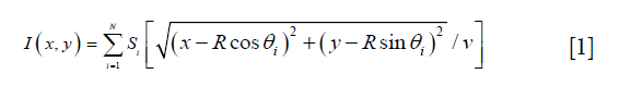

where R is the radius of the transducer scanning trace, N is the number of total transducers, S(t) is the signal received by the i-th transducer, θi is the angular coordinate of the i-th transducer, and v is the acoustic velocity in the media. Eq. [1] can give a uniform resolution for an ideal point transducer, but for a planar transducer with a finite size, the tangential resolution will deteriorate as the imaging point moves away from the circular scanning center, and becomes equal to the transducer size at the boundary of the transducer scanning trace (11).
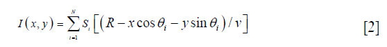
The second expression of the back-projection algorithm is for the transducer to be so big that it is to be regarded as a planar detector with infinite size. The schematic for this situation is shown in Figure 1B, and the projection lines are parallel with the detector plane. The image reconstruction in this case is very similar to the inverse Radon transform, in which the pixel value at (x,y) is given as
However, for a smaller transducer, this equation will also lead to a tangential elongation. Therefore, here we seek to find a concise form of the back-projection algorithm when a transducer with a finite element size is employed. Our strategy is to create a virtual detector, which is located further from the actual transducer, as illustrated in Figure 1C. If the value of the distance between the virtual detector and the actual transducer L is correctly set, the signal received by the transducer Si(t) can be approximate to the signal received by the virtual detector but with a time delay of L/v. In this way, because the radius of the virtual detector scanning trace is R+L, the final pixel reconstruction value that can be given by Eq. [1] becomes
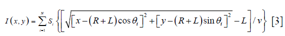
It is also worth noting that in Eq. [3], if L equals to 0, this equation will deteriorate to Eq. [1], which is suitable for ideal point transducers. On the other hand, if on the condition that x2+y2<<R2, meaning if the reconstruction region near the rotation center is much smaller than the scanning radius (so that x and y are infinitely small compared with R+L), the distance delay term in Eq. [3] becomes
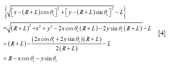
Thus, Eq. [3] becomes
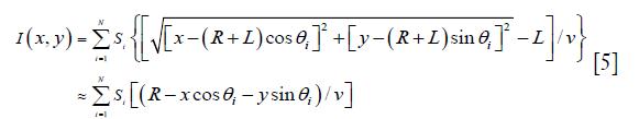
It can be seen here that Eq. [5] gets into the same form of Eq. [2], so it can apply to transducers with infinite element size. Therefore, Eq. [3] represents a universal form of the back-projection method.
Determination of the optimal distance L
Since our strategy is to approximate the acoustic divergence property of the finite size planar transducer with a virtual point detector, the spatial temporal responses of the employed transducer need to be known first, which can be calculated with a linear model that is based on the Fresnel field integral formula as described previously (16). Then, the optimized value of distance L in Eq. [3] is determined using a phase square difference minimization scheme.
Figure 2A shows the proposed scheme. Here, for an arbitrary position A with the coordinate (x,y), the spatial-temporal response can be calculated with the size and frequency response of the employed planar transducer, as shown in Figure 2B. It is apparent that due to the “finite aperture effect” the spatial temporal response of the planar transducer with finite size can be distorted when compared with that of a point detector (9). We regard the signal arrival time of the maximum amplitude in the spatial temporal response to be ΔtA, and for concision, we consider it the signal arrival time, and vΔtA to be the phase of this position A to the transducer. Next, as illustrated in Figure 2A, we expect that the pixels having the same distance to the virtual point detector DisAD (which is the blue curve in the figure) all have the same phase, which means we expect that
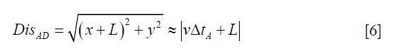

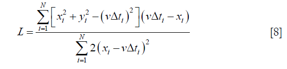
Therefore, if we define a region RA with respect to the transducer (as illustrated in Figure 2A), where most pixels in the reconstruction domain during the CSPAT scan locate, and, if this region is divided into N pixels, then the optimal distance L can be found with the minimum objective in Eq. [7].
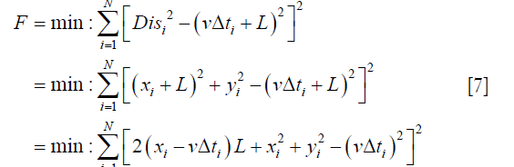
where xi, yi are the coordinates of the i-th pixel in the region RA, and vΔti is the corresponding phase, so that to obtain the differential to Eq. [7] we have
Simulation methods
For the preliminary demonstration of our method, numerical simulation was carried out. In the simulation, there were 4-point targets evenly distributed between 0 to 6 mm on the x axial direction. The planar transducer with a central frequency of 5 MHz, a bandwidth of 70%, and a size of 5 mm was used. The distance between the rotation center and the transducer was 20 mm. There were 360 detectors for a full circular scan, and the angular interval between the detectors was 1 degree. In this simulation, a region was first defined to find the optimal distance L, and the phase distribution and the error distribution were also shown for better illustration. Then, the reconstructed image with our method was compared with those using the two models of the back-projection method. Also, the reconstructed image with the modified back-projection method was also compared to further demonstrate the advantage of our proposed method. In the modified back-projection method, the finite-sized planar detector was modeled as a collection of ideal point detectors, and the final reconstructed value was given by a sum of the delayed signal from the point detectors (12,16), which was the following:
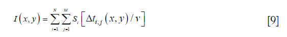
Here, M is the number of ideal point detectors for a transducer, and Δti, j(x,y) is the time delay from the pixel to the point detector. Furthermore, the extracted tangential resolutions for each target represented with full widths at half maximum (FWHMs) were compared between the four methods for a better demonstration. Finally, the influence of the distance L to the final reconstruction results was also studied by comparing the tangential profiles of each target when changing its value.
Phantom experiments
Three phantoms were imaged to test our proposed method. All three phantoms had a diameter of 3 cm for the background, and their scattering and absorption coefficients were 1/mm and 0.007/mm respectively. The first of the phantoms contained 8 pencil leads (0.7 mm thick) as point targets, the second phantom had 5 hairs buried on the top, and the third phantom contained one piece of leaf veins. All three phantoms were successively imaged with a conventional 2D CSPAT system as described elsewhere (1,16). The phantom was given an area of illumination of 5 mJ/cm2 on the top from a Nd:YAG laser (Nimma-600, Beamtech Optronics) with a wavelength of 532 nm. Complete 2D circular scanning was performed in 360 steps and a step size of 1 degree. The employed transducer was a commercial piezoelectric transducer with an aperture size of 5.5 mm, 5 MHz central frequency, 65% bandwidth, and the transducer was placed at about 20 mm distance from the rotation center. The signal from the transducer was first amplified with a pulser/receiver (5072PR, Olympus) and then digitalized with a DAQ card (LDI400SE, DIYANG, 100 MHz sampling frequency). Photoacoustic images were calculated with Eqs. [1], [2], [3], and [9], and compared.
Results
Optimal distance L calculation
As the furthest target was positioned at 6 mm, and the radius of the transducer scanning trace was 20 mm in the simulation, to decide the optimal value of distance L, the region was defined to be 14 to 26 mm in the x direction, and −6 to 6 mm in the y direction. With the central frequency, size, bandwidth of the planar transducer, the spatial temporal response of the planar transducer in this defined region can be calculated, and then the signal arrival time and phase of each pixel in this region can be calculated, as illustrated in Figure 3A. With the calculated phase map, the optimal value of L was calculated to be 22.8 mm. With this value, the phase difference Dis–vΔt was also calculated, as shown in Figure 3B.

Here, the relative position of each pixel to the transducer is indicated. The x axis represents the axial direction of the transducer, and the y axis represents the tangential direction. The values of the two images are both in mm. It can be seen that the contour lines in Figure 3A look concentric, so that the acoustic field of the planar transducer can be approximated with a virtual point detector. Figure 3B shows that the phase difference calculated with the optimal value of L is quite small in most regions (results show that the standard deviation of the phase difference map was only 0.025 mm, compared with the central wavelength of the transducer of 0.3 mm), which means our proposed model is well-suited for the planar transducer. It is also worth noting that since Eq. [6] is always valid on the axis of the transducer, the phase difference is almost zero for regions near the transducer axis.
Simulation reconstruction results
Figure 4A,B,C,D show the images reconstructed with Eqs. [1], [3], [2], and [9] respectively. In Figure 4B, the value of L in Eq. [3] is chosen to be 22.8 mm, as calculated in the previous section. It is clear that for the two points located at 4 and 6 mm, their tangential profiles given by the two conventional models of the back projection algorithm are notably elongated compared with the two points at 0 and 2 mm. However, with Eq. [3] the tangential blurring artifacts are effectively restored. Of further note, although the modified back-projection method also helps to reduce the tangential blur, our proposed method still gives the best results. Additionally, the image with the modified back-projection method showed stronger side lobes for the off-center targets.

For a better illustration, Figure 5 shows the extracted tangential profiles of the four targets located from 0 to 6 mm. Here, the tangential profiles extracted with Eqs. [1], [2], [3], and [9] are indicated with red, blue, green, and black respectively, and the maximum value of each tangential profile is normalized to 1 for comparison. Again, it is plain that for the point targets located at 0 and 2 mm, all the four reconstruction methods give tangential profiles of similar size. However, for the targets located at 4 and 6 mm, the tangential profiles reconstructed with Eq. [3] are much thinner than those reconstructed with Eqs. [1], [2], and [9]. This can also be seen in Table 1, where the FWHMs of the target tangential profiles were acquired as tangential resolution. Results show that for the target located at 6 mm, the FWHM with our proposed method {Eq. [3]} was about 2.1, 1.7, and 1.4 times smaller compared with the results by the Eqs. [1], [2], and [9] respectively.


Full table
To better investigate the influence of the value of L to the tangential resolution in the resulted images, the tangential profile changes of the four targets when changing the value of L were extracted and are shown in Figure 6. The figure shows that the value of L changes, the tangential profile sizes of almost all the off-center targets reduce at first, and then gradually increase. When L is zero, the targets are reconstructed with Eq. [1]; when L is big enough, the situation is close to Eq. [2]. When the value of L is set to be around 23 mm, which is the optimal value predicated with Eq. [8], almost all the targets have the thinnest tangential profiles. The improvement of the tangential resolution is more prominent if the target is further from the rotation center. It is also clear that the change of the tangential profile size is as slow as the change of L, especially for targets not far from the rotation center. Moreover, The target tangential profile reconstructed with Eq. [3] will always smaller than those calculated by using Eq. [1] and Eq. [2]. Therefore, our proposed method is a steady and reliable method for the improvement of tangential resolution in CSPAT.

Phantom experiment results
Figure 7 shows the results for the first phantom experiment. Figure 7A is the photo image of the phantom, and Figure 7B,C,D,E are the images reconstructed with the back-projection method in the forms of the point detector model, finite detector model, and the infinite detector model, and the modified back-projection method respectively. For image reconstruction with Eq. [3], the optimal value of L is calculated to be 28.8 mm for all the phantom experiments. It is quite apparent that because the employed transducer cannot be modeled as an ideal point detector but rather an infinite size planar detector, the off-center targets that reconstructed Eqs. [1] and [2] are notably distorted in the tangential direction, especially those marked by the white arrows in Figure 7B. However, with the finite element size detector model, these artifacts are almost completely resolved. In Figure 7E, it can be seen that although some of the off-center targets are slightly improved in the tangential direction (as indicated with the white arrows in Figure 7E) compared with the results from the ideal-point-detector-based conventional back-projection method in Figure 7B, the modified back-projection method tends to blur the image in the tangential direction due to its strong side lobe effect. For example, the one target encircled in Figure 7E is severely blurred.

Figure 8 gives the results for line target imaging, where we picked one region which is marked with a white circle in Figure 8B for demonstration. It is evident that the hair tip encircled is blurred in the image reconstructed with the ideal point detector model (Figure 8B) and the infinite size detector model (Figure 8D), but Figure 8C indicates a much-improved result. For the modified back projection method, it can be seen that the one hair encircled in Figure 8E is less clear than those in the other three images.

The improvement of the image quality with the finite-size detector model is also demonstrated by the third experiment results in Figure 9. Here, the leaf veins have more complicated structures than the first two phantoms. The image by the finite-size detector model (Figure 9C) is more uniform in the overall image reconstruction quality compared with that by the ideal point detector model (Figure 9B), and is more clear in the image details than the image by the infinite-size detector model (Figure 8D). Moreover, in this piece of leaf vein, there is one vein joint that is not quite notable in the photo image, but shows much stronger absorption in the reconstructed PAT images, which is marked with a white arrow in Figure 9B and circled in Figure 9A. The result given by the finite size detector model shows a much improved profile in the tangential direction over the two other models for this vein joint. Comparatively, Figure 9E shows the worst quality since the image is severely blurred in the tangential direction.

Discussion
The goal of this paper is to develop a more generalized model of the back-projection method for the reconstruction of CSPAT. One merit of CSPAT is that because it has a full view of the imaged target, it can give an isotropic resolution in the resulting image. This is significantly different from the situation in reflection mode imaging, where the lateral resolution is largely elongated, and most features of the target have a small angle with the axial direction of the transducer being poorly reconstructed, which is due to the limited aperture of detection. However, sometimes the tangential resolution for the off-center targets in 2D CSPAT can also be significantly elongated, and part of the reason is a lack of consideration for the influence of the transducer size, along with the inaccurate modeling of the applied reconstruction algorithms.
To improve the tangential resolution in CSPAT, much attention has been drawn to employing positively focused or negatively focused transducers to improve the tangential resolution in CSPAT (12-14); however, planar transducers are still mostly employed because of their good directivity and homogeneity of acoustic field. Matrix-based reconstruction methods can directly take the influence of the detector shape and pulse response function into the model to restore the elongated tangential resolution, but their computational cost is enormous (9). Deconvolution-based algorithms have also been applied, but their robustness needs further investigation (10). Comparatively, the method proposed here inherits the merits of the back-projection algorithm, which is simple, computationally efficient, and robust, and both the simulation and experiments proved that this method can effectively restore the tangential elongation artifacts. It is also noteworthy that while most existing methods for the improvement of tangential resolution in CSPAT are tested experimentally with point targets only, our proposed method is further validated in this work with more complicated targets such as leaf veins.
Although the simulations and experiments above are based on a finite size detector, the expression we have given here is also suitable for an ideal point detector and an infinite size detector, so that it is a more generalized form of the back-projection method. In this proposed method, the optimal value of the adjustable parameter L is closely related to the acoustic field of the employed planar transducer, and we have given equations to calculate its value. Generally, this value would be smaller with a transducer with lower central frequency and small aperture size, since in these conditions the transducer would be more easily modeled as a point detector. Conspicuously, Figure 6 shows that the optimal value is almost identical to targets with different distances to the rotation center, and Figure 3B also shows that with the calculated value, the phase error is small throughout the image. This means that this value is not sensitive to the target positions, or rather the selection of the region for calculating it with Eq. [8]. Even the change of the selected region can slightly change the calculated optimal value of L; the small change of the value would not significantly affect the resulted tangential resolution (Figure 6). Furthermore, compared with the recently reported modified back-projection method, our proposed method here can give thinner tangential profiles, and also show less reconstruction artifacts, an assertion which is validated with both simulations and phantom experiments. As discussed in the introduction section, the modified back-projection method is effective for a large-sized transducer, but as we see it may introduce strong artifacts for a planar transducer with finite size.
Despite the benefits, there are still some disadvantages of our proposed method. For example, due to the limited bandwidth of the transducer and data acquisition system, there is strong noise in the background of the reconstructed images with experimental data. Also, even with our method, the tangential resolution for targets away from the rotation center is still enlarged compared with that around the rotation center (Table 1), so a more advanced method is still needed for further improving the tangential resolution for regions far from the rotation center in CSPAT.
Conclusions
We have proposed a generalized model of the back-projection algorithm, with which the tangential resolution in CSPAT can be effectively improved in case of planar detector of finite size. In this method, the acoustic spatial temporal response of the employed finite size transducer is approximated with a virtual detector placed at an optimized distance behind the transducer, and the optimized distance is determined by a phase square difference minimization scheme. Both the simulations and experiments show that our proposed method can significantly improve the tangential resolution in CSPAT. The proposed method here may guide the experimental design of CSPAT, and be applied in the spherical-scanning-based 3D PAT for human breast imaging.
Acknowledgements
Funding: This work was funded by the National Natural Science Foundation of China (NNSFC) (No. 81501517, 61401520, 31200748).
Footnote
Conflicts of Interest: The authors have no conflicts of interest to declare.
References
- Zhang Q, Liu Z, Carney PR, Yuan Z, Chen H, Roper SN, Jiang H. Non-invasive imaging of epileptic seizures in vivo using photoacoustic tomography. Phys Med Biol 2008;53:1921-31. [Crossref] [PubMed]
- Yang SH, Yin GZ, Xing D. Pharmacokinetic Monitoring of Indocyanine Green for Tumor Detection Using Photoacoustic Imaging. Chin Phys Lett 2010;27:123-6.
- Xi L, Li X, Yao L, Grobmyer S, Jiang H. Design and evaluation of a hybrid photoacoustic tomography and diffuse optical tomography system for breast cancer detection. Med Phys 2012;39:2584-94. [Crossref] [PubMed]
- Xi L, Jiang H. High resolution three-dimensional photoacoustic imaging of human finger joints in vivo. Appl Phys Lett 2015;107:063701. [Crossref]
- Xi L, Jiang H. Integrated photoacoustic and diffuse optical tomography system for imaging of human finger joints in vivo. J Biophotonics 2016;9:213-7. [Crossref] [PubMed]
- Huang N, He M, Shi H, Zhao Y, Lu M, Zou X, Yao L, Jiang H, Xi L. Curved-Array-Based Multispectral Photoacoustic Imaging of Human Finger Joints. IEEE Trans Biomed Eng 2018;65:1452-9. [Crossref] [PubMed]
- Hoelen CG, de Mul FF. Image reconstruction for photoacoustic scanning of tissue structures. Appl Opt 2000;39:5872-83. [Crossref] [PubMed]
- Burgholzer P, Hofer C, Paltauf G, Haltmeier M, Scherzer O. Thermoacoustic tomography with integrating area and line detectors. IEEE Trans Ultrason Ferroelectr Freq Control 2005;52:1577-83. [Crossref] [PubMed]
- Li ML, Tseng YC, Cheng CC. Model-based correction of finite aperture effect in photoacoustic tomography. Opt Express 2010;18:26285-92. [Crossref] [PubMed]
- Roitner H, Haltmeier M, Nuster R, O'Leary DP, Berer T, Paltauf G, Grün H, Burgholzer P. Deblurring algorithms accounting for the finite detector size in photoacoustic tomography. J Biomed Opt 2014;19:056011. [Crossref] [PubMed]
- Xu M, Wang LV. Analytic explanation of spatial resolution related to bandwidth and detector aperture size in thermoacoustic or photoacoustic reconstruction. Phys Rev E Stat Nonlin Soft Matter Phys 2003;67:056605. [Crossref] [PubMed]
- Pramanik M, Ku G, Wang LV. Tangential resolution improvement in thermoacoustic and photoacoustic tomography using a negative acoustic lens. J Biomed Opt 2009;14:024028. [Crossref] [PubMed]
- Song C, Xi L, Jiang H. Liquid acoustic lens for photoacoustic tomography. Opt Lett 2013;38:2930-3. [Crossref] [PubMed]
- Li M, Wang LV. A study of reconstruction in photoacoustictomography with a focused transducer. Proc. SPIE 6437, Photons Plus Ultrasound: Imaging and Sensing 2007: The Eighth Conference on Biomedical Thermoacoustics, Optoacoustics, and Acousto-optics, 64371E (13 February 2007). doi: 10.1117/12.703716. [Crossref]
- Cai D, Li Z, Li Y, Guo Z, Chen SL. Photoacoustic microscopy in vivo using synthetic-aperture focusing technique combined with three-dimensional deconvolution. Opt Express 2017;25:1421-34. [Crossref] [PubMed]
- Xiao J, Luo X, Peng K, Wang B. Improved back-projection method for circular-scanning-based photoacoustic tomography with improved tangential resolution. Appl Opt 2017;56:8983-90. [Crossref] [PubMed]

