

Hierarchical iterative linear-fitting algorithm (HILA) for phase correction in fat quantification by bipolar multi-echo sequence
Introduction
Proton density fat fraction (PDFF) quantification, based on chemical shift-encoded MR imaging techniques, has been validated as an accurate and promising tool to characterize fatty tissue content (1-3). This technique could provide quantitative and spatial information for fat accumulation in a wide range of tissues, including liver (4), skeletal muscle (5), and bone marrow tissue (6).
Chemical shift-encoded imaging is mostly based on multi-echo gradient echo (GRE) sequence. Multi-echo GRE sequence with bipolar readout gradients can reduce the achievable echo spacing time compared to unipolar readout gradients and thus can have higher acquisition efficiency (7). Higher acquisition efficiency is useful for the large coverage required for abdominal imaging acquisitions, in which the ability to complete imaging within a single breath-hold can prevent intra-scan image misregistration. However, in a bipolar readout sequence, an additional phase is modulated to images due to the eddy current arising from the alternating readout gradients (8). The eddy current induced phase (EC-phase) corrupts the phase consistency between the even and odd echoes, making it one of the confounding factors for accurate fat quantification (9).
Many useful approaches have been proposed to address the bipolar readout-induced phase error issue. The EC-phase is dominated by its lower order term and can be approximated to a spatially linear model. The linear order term of the EC-phase can be estimated from either the k-space (8,10) or image space (11,12). Lu et al. (8) proposed a method to estimate the parameters of a linear model by maximizing the cross-correlation coefficient between odd and even echoes after phase compensation. Ruschke et al. (10) measured the k-space shift between odd and even echoes by solving an optimization problem. However, these two methods are limited in the read-out direction. Li et al. (11) estimated the parameters by fitting the linear model to the EC-phase obtained from the phases of the first three echoes. Unfortunately, this estimation may be biased due to fat-containing pixels, as the phase difference between even and odd echoes in the fat containing pixels is no longer equal to the EC-phase, resulting in fat fraction (FF) errors in the far off-center areas. Hernando et al. (12) proposed to fit the parameters in such a way that the fat and water images produced by complex and magnitude signal fittings were best matched after the linear phase terms were removed before the complex signal fitting. However, this method requires numerous calculations to search for the appropriate linear terms.
Several studies have revealed that the higher order term in EC-phase errors results in large fat-water separation and fat quantification errors; therefore, the whole EC-phase needs to be accurately estimated (9,13). Yu et al. (9) corrected phase and amplitude errors by acquiring additional phase-encoded reference lines with a mirrored gradient polarity at each echo. The EC-phase map, including both lower order and higher order terms, and the amplitude inconsistency map, were then estimated through a pair of central k-space data with opposite gradient polarities. Soliman et al. (7) directly averaged the complex images with opposite polarities at each echo to eliminate the eddy current effect before fat-water separation. This method requires two acquisitions with completely mirrored readout gradients and was found to have similar performance to the unipolar acquisition; however, the additional acquisition increases scan time and is not favorable to time-critical applications.
Peterson and Månsson (13) introduced the EC-phase as an unknown factor in the fat-water signal model and solved both the EC-phase and fat-water separation pixel by pixel simultaneously using the IDEAL algorithm. However, in order to implement the IDEAL procedure to solve the field ambiguity problem successfully, an initial guess on the EC-phase must be provided. The initial guess on the EC-phase relies on the complex signals of the first three echoes and the one dimensional (1D) linear phase unwrapping procedure. The joint estimation of the EC-phase and fat-water separation using the IDEAL method easily converges into local minima in regions with strong field inhomogeneity which results in fat-water swaps and consequently inaccurate fat quantification. Additionally, the inclusion of the EC-phase as a free parameter can compromise the SNR performance of fat quantification (7,14).
In this paper, we proposed a simple but practical method to use a hierarchical iterative linear-fitting algorithm (HILA) to correct the nonlinearity of the EC-phase in a bipolar acquisition sequence without additional data acquisition. First, Monte Carlo simulations were completed to evaluate how the EC-phase affects the performance of fat quantification. Then, the accuracy and noise performance of the proposed method were compared to the well-established unipolar acquisition through phantom and in-vivo experiments for validation.
Theory
Signal model
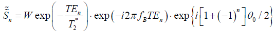
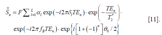
For a multi-echo GRE sequence with N echoes, the signal of a pixel can be represented as a mixture of water and fat complex signals with consideration of the field inhomogeneity fB and the T2* decay effect:
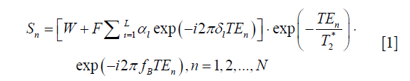
where W and F are water and fat signal intensities, respectively. TEn is the n-th echo time, fB is the local field offset, and N is the total number of echoes. Using a multi-peak fat model, αl and δl are the relative amplitude and chemical shift of the l-th (l = 1, 2, …, L) fat peak to water, and 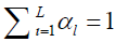 . The single T2* model of fat and water was used in our study (15-17).
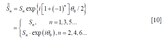
With a bipolar acquisition sequence, the EC-phase θ is modulated to the even echoes. The signal can be then written as the following:
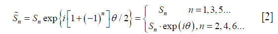
where Sn is defined as Eq. [1].
Eq. [2] can be formulated as a matrix representation:

where S=(S1,..,SN)T, F= diag [exp (–i2πfBTE1),..,exp (–i2πfBTEN)], E= diag <1,..,exp {i [1+(–1)N]θ/2}>, 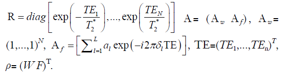
Once T2*, fB, and θ are given, then fat and water complex signals can be given as follows:

When θ is not considered, as in a unipolar acquisition, E becomes an identity matrix. The FF is defined as abs (F)/[abs (W)+abs (F)].
EC-phase estimation
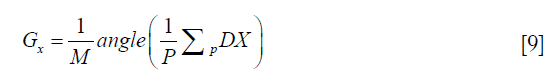
The EC-phase in image domain can be approximated by its low order term when it approaches steady state during data acquisition (5,9,11):
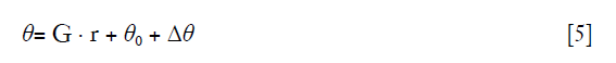
where G = [Gx Gy Gz] is the vector containing the first order coefficients in the physical x/y/z directions respectively, r = [x y z] is the pixel coordinate vector, θ0 is the zero order phase shift, and Δθ is the EC-phase higher order term.
Although the EC-phase can be modeled by higher order polynomials in the image, the fitting process can be unstable due to the limited number of significant digits in the computational system, especially in the areas far from the image center. In this study, a novel EC-phase estimation method is proposed. The nonlinearity of the EC-phase is considered through the stepwise linear fitting under a hierarchical pyramid framework through the whole image.
The flow chart of the proposed algorithm is shown in Figure 1. In each iteration, each image block is divided into sub-blocks, and the EC-phase is fitted to a linear model in each sub-block according to the procedure introduced below. The estimated linear phase in each sub-block is used as a starting value for the next iteration. The pyramid decomposition of the image is terminated until the largest iteration number is achieved or until the stopping conditions for the linear fitting are met in all sub-blocks. Finally, a weighted average over all levels is calculated to obtain the final EC-phase map.

Step 1: fit for the first order term
Supposing the smoothness of the tissue in one direction (taking x as example for generality), water-fat signals, T2*, and the field value fB can be considered to be the same in the neighboring pixels, meaning that

An empirical range is set to detect those pixels which are 0.9 <  < 1.1. Pixels which fail to meet Eq. [6] are usually located in the regions with low signal-to-noise ratio (SNR), or at the tissue-air interface or boundary of water-dominant/fat-dominant tissues. For the pixels satisfying the assumption above, we define:
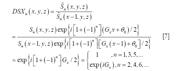
Let:
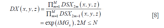
DX becomes independent of spatial position, and Gx can be fitted by the following:
where P is the number of pixels satisfying Eq. [6], p is the index of those pixels, and angle(.) is the phase operator of a complex number.
Similar operations can be done in both y and z directions to obtain Gy and Gz. If the number of pixels satisfying Eq. [6] is less than a preset ratio of the whole pixels (25%), the stopping criterion of this procedure is met, and the subsequent fitting procedure related to the image block is terminated.
Step 2: fit for the zero order term
The first order term of the EC-phase is estimated and removed from Eq. [2], and the signals become as follows:
In pixels that contain only one species (water or fat), the signal of these pixels becomes
or
To find pixels that contain only water or fat, one could either use magnitude fitting (15) or complex fitting (18) from even echoes to find where the FF is approximately 0 or 1. If the number of the pure fat-water pixels is less than a preset ratio of the whole pixels (25%), the stopping criterion of this procedure is met, and the subsequent fitting procedure related to the image block is also terminated.
As equally-spaced TEs (six or more) are commonly used in the multi-echo GRE sequences for fat quantification, we define
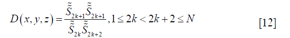
Terms that contain TEn are all canceled out in D, leaving
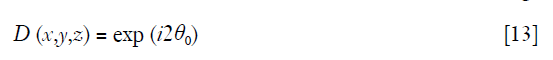
which is spatially invariant. A practical solution of θ0 is
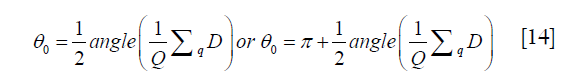
where Q is the number of pixels satisfying Eq. [12], and q is the index of the pixels.
There are two possible solutions which both satisfy Eq. [13]. Although they are equal in the model, the two solutions may produce a π difference in the estimation of the field in Eq. [3]. To ensure consistency and avoid an abrupt field change, the solution which is closer to the starting value (i.e. the linear phase estimated by the parent iteration in the sub-block) is chosen. For the first iteration, the value closest to 0 from the two solutions is chosen as the solution of θ0.
Methods
Monte Carlo simulations
Monte Carlo simulation data were created to investigate the presence of the residual EC-phase and how it would affect the accuracy of FF quantification. The simulated data were generated using Eq. [2]. A six-peak spectrum of fat was used (19). The remaining EC-phase (θ) ranged from [−π/2, π/2] with a step π/60; TE1 was fixed to 1.78 ms, echo spacing ΔTE ranged from 0.1 to 2.2 ms, FF ranged from [0–1] with a step of 0.1, fB was set to 40 Hz, and single T2* =50 ms. For each combination of parameters, 2,500 groups of multi-echo data were generated. Random Gaussian noise was added to the data with SNR =50 (signal intensity at TE =0 to noise ratio). The simulated data were then processed under the signal model in Eq. [1] without the EC-phase considered. Then FF was computed according to the estimated W and F. The mean error of the FF estimation relative to the true value was derived to describe the effects of the residual EC-phase.
Phantom study
The accuracy of the proposed EC-phase estimation method for FF quantification was validated through phantom experiments. Fat-water phantoms with FFs of 10%, 20%, 30%, 40%, and 50% were constructed (12,20). The nominal FF of the phantoms are defined as the fat volume percentages (21). Briefly, the phantoms were constructed by the following steps: deionized water, agar (2% w/v), sodium dodecyl sulfate (SDS, 43 mM), sodium chloride (43 mM) and sodium benzoate (3 mM) (Sigma Aldrich, St. Louis, MO) were mixed in a glass beaker and heated in a microwave oven until boiling. The solution and peanut oil were then poured into 20-mL scintillation vials with a predetermined volume ratio. They were mixed through gentle inversion for approximately 2 min. Last, the vials were immersed in ice for 30 min to form gel. Along with a pure peanut oil phantom, the 6 phantoms were put into a tank filled with water.
MR scans were conducted on a Siemens TIM Trio 3T system (Siemens, Erlangen, Germany). Before acquiring the bipolar datasets, a unipolar readout dataset was acquired as a reference for FF quantification. A 3D multi-echo GRE sequence was used for both the unipolar and bipolar acquisitions with the following parameters: TR =30 ms, matrix =192×192, imaging resolution =2×2×2 mm3, bandwidth =2,003 Hz/pixel, number of average =5, and acquisition time =461 s. A small flip angle (FA =3°) was used to mitigate the T1 effect (22). For both the unipolar and bipolar acquisitions, the first TE was fixed to 1.78 ms with ΔTE =1.95 ms, which was the minimal echo spacing achievable for the unipolar acquisition. Two other ΔTEs were adopted for bipolar acquisitions: ΔTE =0.96 ms, which was the minimal echo spacing achievable for bipolar acquisition, and ΔTE =1.50 ms. For the bipolar acquisition, imaging slices were firstly set in a coronal orientation (Normal Slices, NS). Then, the imaging plane was rotated 45° in-plane for an oblique acquisition (Oblique Slices, OS). In both acquisitions the phantoms were scanned once in the left side of the water tank, once in the center of the water tank, and once in the right side of the water tank, for a total of 3 times per acquisition. Eighteen groups of bipolar datasets were ultimately collected in the phantom study (combination of 3 ΔTEs, 2 orientations, and 3 positions). Temperature-induced water frequency shifts were carefully calibrated through a fluorescent thermometer; chemical shift of fat peaks were corrected accordingly (14,23).
Human study
This portion of the study was approved by the local Institutional Review Board (IRB), and informed consent was obtained from all three participants. The body mass indices (BMIs) of the three volunteers were 23.5, 27.8, and 32.7 kg/m2. To demonstrate the performance of the proposed method on MR systems from different vendors, participants underwent upper abdominal scans with a six-echo 3D GRE sequence on two 3T MR systems: Siemens TIM TRIO (Siemens, Erlangen, Germany) and UIH uMR 790 (Shanghai United Imaging Healthcare, Shanghai, China). Both bipolar and unipolar datasets of axial and coronal orientations were acquired with breath-hold. The common parameters were as follows: TR =14 ms, first echo time =1.78 ms, imaging resolution =3×3 mm2, slice thickness =5 mm, FA =3°, readout bandwidth =1,950 Hz/pixel, and matrix =128×108 for axial acquisitions and 128×128 for coronal acquisitions. The acquisition time was ~19 s. The minimal echo spacing was set for unipolar and bipolar acquisition as ΔTE =1.56/0.92 ms for TIM TRIO, and ΔTE =1.48/0.74 ms for uMR 790.
Data processing
All data were processed in MATLAB (Natick, MA, USA). Each bipolar dataset was processed in the following way:
- The EC-phase was estimated by our proposed method with maximal iteration = 10. The estimated EC-phase was removed from the original data.
- Data were then applied to the region growing with self-feeding algorithm proposed in (21). The parameters of W, F, f, and T2* were derived.
- The FF was computed with noise correction (20).
For the unipolar dataset, only the latter two steps were applied; the resulting FFs were used as the reference.
For the phantom data, FFs were obtained by placing ROIs on each of the 5 (FF =10%, 20%, 30%, 40%, and 50%) fat-water phantoms over the central 3 slices. ROIs were also placed on the 4 corners of the water tank, which were recorded as pure water (FF =0%), and the tube with only oil (FF =100%). For the tubes with FF =10%, 20%, 30%, 40% and 50%, the unipolar results were used as reference. For the tubes with pure oil and pure water area, FF =100% and 0% respectively, were used as references.
For the human data, 3 ROIs were placed on the liver, and 1 ROI was drawn on the subcutaneous fatty tissue on axial images. On the coronal acquisitions, 2 ROIs were placed on the liver, and 2 ROIs were placed on the subcutaneous fatty tissue. The ROIs in the liver were selected in such a way as to avoid large blood vessels or any liver lesions. The mean FF and standard deviation (SD) were calculated across all ROIs for the unipolar acquisitions and bipolar acquisitions.
Results
Monte-Carlo simulations
Figure 2 shows the FF error maps in terms of the absolute mean (Figure 2A) and SD (Figure 2B) due to the EC-phase error. When ΔTE is approximately 0.95, 1.5, or 1.95 ms, the FF estimation is relatively robust to the residual EC-phase, as the largest mean FF errors are small (<2%) under these ΔTEs. However, when choosing ΔTE around 1.15 ms, at which fat and water have opposite phases, the FF estimation becomes vulnerable to the EC-phase residual. The error curves of Figure 3 indicate that as long as the residual EC-phase estimation can be limited to π/8 with ΔTE =0.95 or 1.5 ms, the FF estimation error can be rather small (~2%) for FF =0, 50% and 100%. The estimation error with ΔTE =1.50 ms is slightly smaller than the error with ΔTE =0.95 ms, and the error is smaller with FF =100% for both ΔTEs.


Phantom study
The averaged FF values estimated from the unipolar dataset were 11.5%, 18.4%, 33.6%, 42.6% and 52.7% for the phantoms with FF =10%, 20%, 30%, 40%, and 50% respectively, and the measured FF were used as reference for the latter comparison results.
Figure 4 show the EC-phase estimation results from the linear model method (10) and the proposed method. The original multi-echo data were obtained by bipolar acquisition with ΔTE =0.96 ms for oblique scans. Figure 4A,B,C,D show the EC-phase images derived from the linear fitting method (Figure 4B) and the proposed method with iteration =4, 7 and 10 (Figure 4B,C,D) respectively. The results show that there exists higher order term in the EC-phase, and that the linear model is not accurate enough for the description of the EC-phase distribution, especially in the areas far away from the image center. Figure 4E,F,G,H show the FF estimated from the linear model method and the proposed method with different iterations. There exists significant FF error with the linear model method. For the proposed method, with pyramid decomposition of the image into smaller sub-blocks, the FF estimation error decreases and the distribution of FF in pure water region is uniform with iteration =10.

Figure 5 shows FF estimations of all 18 bipolar acquisitions. The mean FFs of these acquisitions were 0.36%, 11.2%, 18.8%, 33.5%, 42.4%, 52.5% and 100.1%. The differences between these values and the reference FFs were 0.36%, −0.26%, 0.35%, −0.09%, −0.15%, −0.21%, and 0.09%.

Figure 6 gives the linear regression between the reference FF and the FF values estimated from the bipolar acquisitions with normal orientation, but different phantoms locations and ΔTEs. The linear regression results show that FF estimated from bipolar acquisitions agreed closely with reference FF.

Bland-Altman analyses gives the mean FF differences of the three ΔTEs estimated from normal and oblique acquisitions at the three phantoms locations (Figure 7). No significant differences were found.

Figure 8 shows the FF mean error in each tube to the unipolar results with ΔTE =0.96 ms and ΔTE =1.50 ms. The results show that the absolute FF mean errors were smaller than 1.0% for most of the tubes when the tubes were aligned in the right, middle, or left side of the water tank on both normal and oblique slices. Interestingly, the total mean error was smaller with ΔTE =1.50 ms than with ΔTE =0.96 ms. The results are consistent with the simulation results in Figure 3.

Human study
Figure 9 shows the phase images of the second TE from unipolar and without/with EC-phase corrected bipolar acquisitions. The phase evolution of a pure water pixel and final FF maps confirm that the phase inconsistency between the odd/even echoes was removed.

Abdominal FF maps from unipolar and bipolar acquisitions of the volunteer with the highest liver FF are shown in Figure 10. There are no significant differences or obvious fat-water swaps in the bipolar acquisition FF maps compared to the unipolar acquisition FF maps.

Table 1 gives the means and SDs of the FFs within the ROIs in the liver and subcutaneous fat tissue for all three volunteers, which are calculated from the proposed method using both unipolar and bipolar acquisitions scanned from two MR systems. As shown in the Table 1, the accuracy of the proposed method is comparable to the unipolar acquisition. The minimal/median/maximal FF differences between these unipolar and bipolar acquisitions for the three volunteers are 0.6%/1.2%/2.2%, 0.3%/1.1%/1.9%, and 0.2%/0.75%/1.5% respectively. A linear regression analysis shows that the noise performance is not compromised and that there is no significant FF difference between the two different MR systems (r2=0.9994 and RMSE =1.0%).

Full table
Discussion
In this study, we proposed an EC-phase correction method for bipolar acquisition sequences. Despite the linear EC-phase terms, we used a stepwise linear fitting method to approximate the high-order terms. We also investigated the quantitative relationship between the residual EC-phase after correction and the accuracy of FF estimation through simulation.
The phantom study showed that the proposed EC-phase correction method resulted in consistent FF estimation regardless of the imaging orientation and only produced a small FF error compared to the unipolar results (see Figures 6-8). These findings imply that the proposed method is robust for fat quantification on a bipolar acquisition regardless of image location, orientation, and ΔTE, which is beneficial for the in vivo study where higher acquisition efficiency is required (24). Furthermore, the proposed method is useful for images with oblique orientations, such as the shoulder (25), heart (26), or locations where the EC-phase is found to be larger and more complicated than expected due to anisotropic gradient behavior of the gradient delay between different gradient coils (9).
The EC-phase corrupts the phase consistency between odd and even echoes in multi-echo GRE sequence with bipolar acquisition, which is a common problem for the applications using the phase information from the multi-echo sequence (11). However, in fat quantification, the EC-phase estimation problem is more complicated as the whole image cannot be assumed to be pure water or water-dominant. As a result, the method in Ref (11) might not be applicable. EC-phase could be either estimated through k-space data by aligning the k-space center between odd and even echoes (10). This method is equivalent to the linear estimation of EC-phase in image domain. However, a linear model over the whole image might be insufficient especially in the off-center areas of the image. The phantom experiment results show that there might exist a high degree of FF error if only the low-order terms are considered.
The EC-phase could be estimated by acquiring additional readout lines with the opposite readout gradients (9). Low resolution image pairs from the opposite readout lines were used for EC-phase estimation in image domain. Soliman et al. even proposed to acquire the whole k-space lines to cancel out the effect of EC-phase (7). However, the additional acquisition increases the scan time, and is not favorable to time critical application, such as in liver fat quantification.
In the study of Peterson and Månsson, by incorporating the EC-phase into the chemical shift encoded signal model, the EC-phase could be accurately estimated pixel by pixel together with the fat/water separation (13). However, in order to implement IDEAL procedure to solve the field ambiguity problem successfully, an initial guess on the EC-phase should be provided. The initial guess on EC-phase relies on the complex signals of the first three echoes and one-dimensional (1D) linear phase unwrapping procedure. However, as stated by Soliman et al. (7), the employed 1D linear phase unwrapping might be insufficient for 2D phase wraps in clinical applications. In the proposed method, the EC-phase is approached by a 2D stepwise linear fitting procedure with no need for phase unwrapping. The following fat/water separation is completed by our previous proposed method which is more robust when applied to regions with strong field inhomogeneity (18).
Although various EC-phase correction methods have been proposed, the quantitative relationship between residual EC-phase and FF estimation is not well established to the best of our knowledge. Through Monte Carlo simulations, we found that some ΔTEs (i.e., ~0.80/1.50/1.95 ms) are more favorable than others for accurate FF estimation in the presence of a moderate residual EC-phase ranging from −2π/15 to 2π/15 (Figures 2,3). These ΔTEs may result in small FF estimation errors because they correspond to inter-echo fat-water phase shifts ~4π/6, ~8π/6, and ~10π/6 for 6-echo data at 3 T, meaning the average between the even/odd echoes might cancel out the EC-phase effect on FF estimation. For example, when ΔTE =1.5 ms, the fat-water phase shift to the first echo is 0, 4π/3, 2π/3, 0, 4π/3, and 2π/3 for the 6 echoes. The even/odd echo pairs have the same inter-echo phase shift: 0, 2π/3 and 4π/3, which are quite similar to acquiring three echo data twice with completely opposite readout polarities. Therefore, ΔTEs satisfying the above relationship between even/odd echoes are a recommended choice for bipolar acquisitions. It is important to note that when ΔTE ~1.15 ms, at which fat and water have opposite phases, FF estimation became vulnerable to the EC-phase. Ref (13) explains that this phenomenon occurs because the modulation frequency of the EC-phase and the fat main-peak on acquired signals are the same, resulting in ambiguity of these two factors.
The current study only corrects the phase error induced by eddy current and does not address the amplitude error between even and odd echoes. Previous studies have suggested the need to correct the amplitude error (9). The lack of significant differences between the bipolar and unipolar datasets in both our phantom and human studies suggest that addressing the amplitude error is not imperative. Nevertheless, the amplitude error between echoes will be investigated in future studies.
Conclusions
In the present study, we investigated the influence of the EC-phase on the accuracy of FF quantification and proposed a simple and efficient EC-phase correction method for bipolar acquisition using a hierarchical linear fitting algorithm (HILA). Monte Carlo simulations demonstrated that the fat quantification results were robust to the EC-phase for certain ΔTEs. The performance of this method was further validated by phantom and human experiments using the unipolar acquisitions as references.
Acknowledgements
Funding: This research was supported by the Natural Science Foundation of China (Nos. 81327801, 81527901, 11504401 and 81801724), the Key Laboratory for Magnetic Resonance and Multimodality Imaging of Guangdong Province (No. 2014B030301013), and the Shenzhen Science and Technology Research Program (No. JCYJ20170413161350892).
Footnote
Conflicts of Interest: The authors have no conflicts of interest to declare.
Ethical Statement: The study was approved by the local Institutional Review Board (IRB) and written informed consent was obtained from all patients.
References
- Hu HH, Börnert P, Hernando D, Kellman P, Ma J, Reeder SB, Sirlin C. ISMRM workshop on fat–water separation: insights, applications and progress in MRI. Magn Reson Med 2012;68:378-88. [Crossref] [PubMed]
- Idilman IS, Aniktar H, Idilman R, Kabacam G, Savas B, Elhan A, Celik A, Bahar K, Karcaaltincaba M. Hepatic steatosis: quantification by proton density fat fraction with MR imaging versus liver biopsy. Radiology 2013;267:767-75. [Crossref] [PubMed]
- Yokoo T, Bydder M, Hamilton G, Middleton MS, Gamst AC, Wolfson T, Hassanein T, Patton HM, Lavine JE, Schwimmer JB. Nonalcoholic fatty liver disease: diagnostic and fat-grading accuracy of low-flip-angle multiecho gradient-recalled-echo MR imaging at 1.5 T. Radiology 2009;251:67-76. [Crossref] [PubMed]
- Meisamy S, Hines CD, Hamilton G, Sirlin CB, McKenzie CA, Yu H, Brittain JH, Reeder SB. Quantification of hepatic steatosis with T1-independent, T2*-corrected MR imaging with spectral modeling of fat: blinded comparison with MR spectroscopy. Radiology 2011;258:767-75. [Crossref] [PubMed]
- Peterson P, Romu T, Brorson H, Dahlqvist Leinhard O, Månsson S. Fat quantification in skeletal muscle using multigradient-echo imaging: Comparison of fat and water references. J Magn Reson Imaging 2016;43:203-12. [Crossref] [PubMed]
- Gee CS, Nguyen JT, Marquez CJ, Heunis J, Lai A, Wyatt C, Han M, Kazakia G, Burghardt AJ, Karampinos DC. Validation of bone marrow fat quantification in the presence of trabecular bone using MRI. J Magn Reson Imaging 2015;42:539-44. [Crossref] [PubMed]
- Soliman AS, Wiens CN, Wade TP, McKenzie CA. Fat quantification using an interleaved bipolar acquisition. Magn Reson Med 2016;75:2000-8. [Crossref] [PubMed]
- Lu W, Yu H, Shimakawa A, Alley M, Reeder SB, Hargreaves BA. Water–fat separation with bipolar multiecho sequences. Magn Reson Med 2008;60:198-209. [Crossref] [PubMed]
- Yu H, Shimakawa A, McKenzie CA, Lu W, Reeder SB, Hinks RS, Brittain JH. Phase and amplitude correction for multi-echo water–fat separation with bipolar acquisitions. J Magn Reson Imaging 2010;31:1264-71. [Crossref] [PubMed]
- Ruschke S, Eggers H, Kooijman H, Diefenbach MN, Baum T, Haase A, Rummeny EJ, Hu HH, Karampinos DC. Correction of phase errors in quantitative water–fat imaging using a monopolar time-interleaved multi-echo gradient echo sequence. Magn Reson Med 2017;78:984-96. [Crossref] [PubMed]
- Li J, Chang S, Liu T, Jiang H, Dong F, Pei M, Wang Q, Wang Y. Phase-corrected bipolar gradients in multi-echo gradient-echo sequences for quantitative susceptibility mapping. MAGMA 2015;28:347-55. [Crossref] [PubMed]
- Hernando D, Sharma SD, Aliyari Ghasabeh M, Alvis BD, Arora SS, Hamilton G, Pan L, Shaffer JM, Sofue K, Szeverenyi NM. Multisite, multivendor validation of the accuracy and reproducibility of proton-density fat-fraction quantification at 1.5 T and 3T using a fat–water phantom. Magn Reson Med 2017;77:1516-24. [Crossref] [PubMed]
- Peterson P, Månsson S. Fat quantification using multiecho sequences with bipolar gradients: investigation of accuracy and noise performance. Magn Reson Med 2014;71:219-29. [Crossref] [PubMed]
- Hernando D, Sharma SD, Kramer H, Reeder SB. On the confounding effect of temperature on chemical shift-encoded fat quantification. Magn Reson Med 2014;72:464-70. [Crossref] [PubMed]
- Hernando D, Liang ZP, Kellman P. Chemical shift–based water/fat separation: A comparison of signal models. Magn Reson Med 2010;64:811-22. [Crossref] [PubMed]
- Horng DE, Hernando D, Hines CD, Reeder SB. Comparison of R2* correction methods for accurate fat quantification in fatty liver. J Magn Reson Imaging 2013;37:414-22. [Crossref] [PubMed]
- Reeder SB, Bice EK, Yu H, Hernando D, Pineda AR. On the performance of T2* correction methods for quantification of hepatic fat content. Magn Reson Med 2012;67:389-404. [Crossref] [PubMed]
- Cheng C, Zou C, Liang C, Liu X, Zheng H. Fat-water separation using a region-growing algorithm with self-feeding phasor estimation. Magn Reson Med 2017;77:2390-401. [Crossref] [PubMed]
- Reeder SB, Sirlin CB. Quantification of liver fat with magnetic resonance imaging. Magn Reson Imaging Clin N Am 2010;18:337-57. [Crossref] [PubMed]
- Hines CD, Yu H, Shimakawa A, McKenzie CA, Brittain JH, Reeder SB. T1 independent, T2* corrected MRI with accurate spectral modeling for quantification of fat: Validation in a fat-water-SPIO phantom. J Magn Reson Imaging 2009;30:1215-22. [Crossref] [PubMed]
- Reeder S, Hines C, Yu H, McKenzie C, Brittain J. editors. On the definition of fat-fraction for in vivo fat quantification with magnetic resonance imaging. 17th meeting of the international society of magnetic resonance in medicine. 2009.
- Liu CY, McKenzie CA, Yu H, Brittain JH, Reeder SB. Fat quantification with IDEAL gradient echo imaging: correction of bias from T1 and noise. Magn Reson Med 2007;58:354-64. [Crossref] [PubMed]
- Cheng C, Zou C, Wan Q, Qiao Y, Pan M, Tie C, Liang D, Zheng H, Liu X. Dual-step iterative temperature estimation method for accurate and precise fat-referenced PRFS temperature imaging. Magn Reson Med 2019;81:1322-34. [Crossref] [PubMed]
- Zhong X, Nickel MD, Kannengiesser SA, Dale BM, Kiefer B, Bashir MR. Liver fat quantification using a multi-step adaptive fitting approach with multi-echo GRE imaging. Magn Reson Med 2014;72:1353-65. [Crossref] [PubMed]
- Lee YH, Kim S, Lim D, Song HT, Suh JS. MR quantification of the fatty fraction from T2*-corrected Dixon fat/water separation volume-interpolated breathhold examination (VIBE) in the assessment of muscle atrophy in rotator cuff tears. Acad Radiol 2015;22:909-17. [Crossref] [PubMed]
- Börnert P, Koken P, Nehrke K, Eggers H, Ostendorf P. Water/fat-resolved whole-heart Dixon coronary MRA: An initial comparison. Magn Reson Med 2014;71:156-63. [Crossref] [PubMed]

