

Acoustic field simulation method for arbitrarily shaped transducer with dynamically refined sub-elements
Introduction
The ultrasound transducer plays an important role in acquiring high quality results with ultrasonic or photoacoustic systems. In many cases, sophisticated transducer aperture designs are employed to create special ultrasound fields for industrial or biomedical applications (1). Before the building of these transducers, computer simulation is strongly needed to characterize and optimize their acoustic properties.
So far, considerable efforts have been made to develop acoustic field simulation algorithms with high accuracy and efficiency. Among these algorithms, the numerical solution of the time domain acoustic wave propagation equation using finite-difference method is a flexible way to obtain the acoustic field (2-4), because it works for both linear and non-linear acoustic fields. However, the discretization of the differential equation and the subsequent large matrix solution involved in this method are highly time consuming and should be treated with great caution to avoid numerical instability issues (5). Moreover, an extra absorption boundary is required in this method (5). Consequently, the methods based on spatial impulse response (SIR) are usually adopted as an effective alternative choice (6-8). These methods calculate the emitted acoustic field by convoluting the SIR of the transducer aperture with the excitation pulse, under the assumption that the acoustic field is linear. The exact analytical solution of SIR has been found for several regular transducer aperture shapes (6,9), but there is no analytical solution for arbitrarily shaped transducers or transducers with heterogeneous distributions of apodization/excitation delay (10,11). Therefore, for most cases, the methods based on sub-elements (SE) are employed to find the SIR of the transducer numerically (5,10-13). These methods approximate the SIR of the transducer aperture with the accumulation of a series of SIRs of simple-shaped SEs which the transducer aperture is divided into. In these kinds of methods, the SIR of a SE can be calculated by using its area and central coordinates (direct SE, DSE) (5,11,14), or by tracking the time trace of SIR inside the SE (time tracing SE, TTSE) (10,12). For the former, the distance from any region in a SE to a field point (FP) is taken to be invariant. To satisfy this approximation, the size of the SE needs to be quite small, so the number of SEs is very large, which leads to an enormous time expenditure and memory cost when employing this method. In the latter method, the SIR of a SE is sampled at a series of time points which are determined by the sampling frequency. Then, a trapezoidal integral is employed to convolute these sampling values of SIR with the excitation pulse in order to get the acoustic pressure (AP). Because the SIR of a SE can have drastic and nonlinear changes due to its edges, and SIR is assumed to change linearly between adjacent sampling time points, a high sampling frequency is required to ensure the accuracy of the trapezoidal integral in this case.
In this work, we propose a new method based on the dynamic refined SE method to calculate the acoustic field of the arbitrarily structured transducers. Just like other SE-based methods, the aperture of the transducer is first divided into triangular SEs in this method. Then, each triangular SE is dynamically segmented into several sub-parts (SPs). The number of SPs in a SE is decided by the flight time of the FP-centered spherical wave across the SE and the sampling frequency. To obtain the SIR for each SP, the slowly changed flight time from the transducer aperture to a FP is approximated with a step function in a SE, and the fast changed length of intersection between the SE and FP-centered spherical wave (LISFSW) is evaluated by the area of the SP. Finally, the SIR of all the SPs are convoluted with the excitation pulse and summed up to get the AP.
Methods
If the media is homogeneous and bounded, and the pressure is small enough that the linearity constrain condition can be met, the AP emitted by a transducer can be described with the equation below (14):
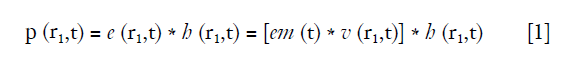
where r1 denotes the location of a FP, * represents the time convolution, v (r1,t) is the input voltage signal to the transducer, em (t) is the electro-mechanical impulse response, e (r1,t) is the excitation pulse, and h (r1,t) is the SIR of the transducer aperture that is decided by its three-dimensional geometry, and can be described by Eq. [2] (15):
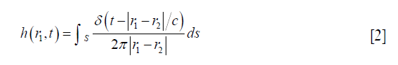
where c is the speed of sound, r2 is a position on the transducer aperture, and S, δ (·) is the Dirac delta function. In Eq. [1], e (r1,t) is usually predefined, so the simulation work is mainly to calculate SIR h (r1,t). In Eq. [2], the SIR of the transducer relative to a FP at r1 is determined by summing the spherical waves originating from all of the positions in the transducer aperture which satisfy |r1–r2|/c = t. According to reciprocity principle, this summing also can be taken as the length of the intersection between the transducer aperture and the spherical wave centered at r1 with its radius satisfying |r1–r2|/c = t. The SIR of a transducer’s aperture can be divided with triangular SEs. Compared to SEs with other geometries, triangular SE is more effective in approximating the complex geometry of the transducer aperture. However, as reported by Jensen (16), the SIR of a SE could have drastic and nonlinear changes. These changes generate very high frequencies in the short responses from small SEs, so the SIR of a SE is difficult to handle in a sampled simulation algorithm. In the conventional TTSE methods, the SIR of a SE is sampled according to the sampling frequency. Then, a trapezoidal integral is employed to convolute these sampling values of SIR with the excitation pulse to generate the AP. Since the SIR of a SE can have drastic and nonlinear changes due to its edges, and the SIR is assumed to change linearly with a constant gradient between adjacent sampling time points in a trapezoidal integral, a high sampling frequency is required in this method to ensure the accuracy of simulation.
Because the time duration of the generated AP signal is determined by the simulation region and fixed, the total number of sampling time points is proportional to the sampling frequency. At each time point, the value of SIR of the SE needs to be calculated. Therefore, the calculation cost for the final SIR is proportional to the sampling frequency. Moreover, the time cost of the convolution between the SIR and the excitation pulse is proportional to the second power of the sampling frequency. As a result, a high sampling frequency can decrease the calculation efficiency significantly.
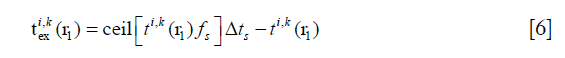
To fix this problem, a method based on the dynamically refined SEs is proposed here. With a constant acoustic speed, the SIR is determined by two terms: (I) the aperture-PF distance |r1–r2|, (II) the length of the intersection between the transducer aperture and the spherical wave centered at r1 with its radius satisfying |r1–r2|/c = t. Since |r1–r2| is far larger than the size of a SE in the far field, the variation of |r1–r2|inside an SE is small. On the other hand, the LISFSW can drastically change due to the edges of an SE, which causes sharp and nonlinear changes in the SIR of an SE. In the proposed method, each SE is further segmented by a series of parallel arcs which are centered at the projection of point r1 on the plane of the SE, as shown in Figure 1. The regions divided by the concentric arcs are named SPs. Because the computational burden of refining the operation is quite small compared with the other parts of the algorithm, this refining operation will not increase the total time consumption significantly. The number of SPs  for the i-th SE and the FP at r1 is given by the following equation:
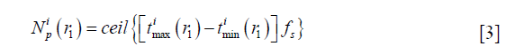

where  and
and  are the maximum and minimum flight time from the SE i to the FP at r1, and fs is the sampling frequency. ceil (·) means round to the next larger integer. The SE is divided by the arcs to make the flight time interval, Δ|r1–r2|/c, between adjacent arcs the same. With a proper sampling frequency and aperture-FP distance, Δ|r1–r2|/|r1–r2| will be small enough to be neglected in an SP. Under the assumption that |r1–r2| is invariant in an SP, the SIR for an SE is rewritten as follows:
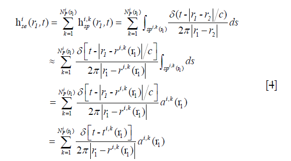
where  is the SIR of the i-th SE related to the FP at r1,
  is the SIR of the k-th SP in the i-th SE, and αi,k (r1), and ri,k (r1) are the area and central location of the SP, respectively. Although |r1–r2| changes slowly in an SE, the LISFSW changes fast and nonlinearly with |r1–r2|, which causes the drastic and nonlinear variation of SIR. As a result, a high sampling frequency is required if a series of sampling values is employed to evaluate the SIR of an SE. In the proposed method, the slowly changed |r1–r2| is approximated by a step function in an SE, so the LISFSW in Eq. [4] can be evaluated by the areas of the corresponding SPs. In each SP, Δ|r1–r2|≤ c/fs, Δ|r1–r2|/|r1–r2|≤ c/ (fs|r1–r2|) can be met in the proposed method. Instead of sampling a drastically and nonlinearly changed SIR of the SE, the sampling frequency in the proposed method only needs to make c/ (fs|r1–r2|) far less than 5%. In a far field, a relatively low sampling frequency will work, thus a significantly lower sampling frequency can be used in the proposed method than one in a TTSE.
Next, the AP emitted by a SP is calculated based on its SIR, which is the following:
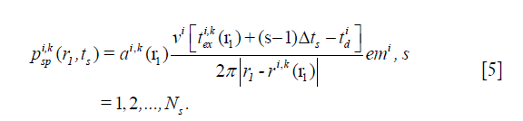
where ts is the s-th sampling time point, Ns is the sampling length of excitation pulse, Δts = 1/fs,  and emi are the excitation delay and electro-mechanical impulse responses of the i-th SE;
  is given by the following equation:
The total AP generated by the whole transducer aperture can be obtained by adding the APs from all the SPs together. The acoustic field value of r1 is given by the max amplitude of the AP emitted by the aperture to r1.
Results
To evaluate the performance of the proposed method, the acoustic field from two different transducers are calculated with our proposed method and Field II. As a widely used TTSE-based software, the effectiveness of Field II has already been proven in experiments (16). The accuracy of the generated data in Field II can be severely degraded by a low sampling frequency, thus a fairly high sampling frequency (1,024 times higher than the central frequency of the transducer) is used to generate the benchmark. The proposed method in the work is implemented in C++, and the Field II is executed by calling the C++ library functions in an official package (version 3.24). In the simulations, the input voltage signal v (r1, t) is a sine function with 2 cycles. The transducer’s electro-mechanical impulse response em (t) is defined by a sine function of 2 cycles filtered by a hamming window whose length is also 2 cycles. The simulations were run on a PC with 64 GB RAM and Intel Xeon E5-2640 CPU. For results comparison, mean relative error (MRE) is employed to evaluate the deviation of the simulation result from the benchmark data. The MRE is calculated with the following equation:
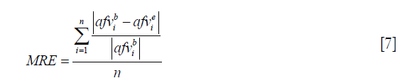
where  and
and  indicate the i-th acoustic field value from the benchmark data and the evaluated simulation results, respectively; n is the length of the data.
In the first simulation, the acoustic field from a transducer array is calculated. As shown in Figure 2, the array is composed of 64×16 rectangular elements in its height and width direction (z and y direction), with an element size of 1 and 2 mm, and a total size of 67.5 and 32 mm, respectively. The array elements are shaped into an arc on the x-y plane to focus the emitted acoustic field on the line of (x=128, y=0) mm. The focus on the z direction is controlled by the excitation delay of the elements. There are two foci located at (x=16, y=0, z=15) mm and (x=16, y=0, z=–5) mm, which are formed by the elements in the upper half and the lower half of the array simultaneously. The central frequency of each element is 5 MHz. The whole array aperture is divided into 8,192 triangular SEs. The geometrical and excitation delay information of the array is also presented in Figure 2. The acoustic field is calculated in the plane defined by 108 ≤ x ≤ 148, –20.0 ≤ z ≤ 20.00 and y=0.0 mm. With a pixel resolution of 0.25 mm, 25,921 FPs are included in this region. The benchmark data provided by Field II is based on a sampling frequency of 5.12 GHz, and the simulation results of the proposed method have a sampling frequency of 80 MHz. For comparison, another simulation is also done with Field II under a sampling frequency of 80 MHz. All the three simulation results are shown in Figure 3. It can be seen that the results given by our proposed method are similar with the benchmark data. However, with the same 80 MHz sampling frequency, the calculated acoustic field by Field II shows some obvious stripped discontinuities. Comparatively, although with a much lower sampling frequency, the acoustic field with our proposed method is as smooth as the benchmark data, and is almost artifact free. The data on several checking lines (x=118, x=128, z=−5 and z=15 mm) are evaluated and shown in Figure 4. Figure 4A and 4B indicate that the acoustic field of the 80 MHz Field II result has a slightly lower intensity compared with the benchmark data near the two foci. Furthermore, abnormal perturbations caused by the stripped artifacts and discontinuous flaws are also observed in the 80 MHz Field II data on the checking lines of z=−5 and z=15 mm, as shown in Figure 4C and 4D. Comparatively, the data from our proposed method matches excellently with the benchmark data on all the four checking lines. The MRE relative to the benchmark data are also calculated for the data on each checking line, as shown in Table 1. The MREs of the result generated by our proposed method are 10 to 20 times smaller than those of the Field II result which is generated with the same sampling frequency.


Full table
In the second simulation, the acoustic fields of a hollow focused transducer with the two methods were compared. As shown in Figure 5, the focal length and diameter of the transducer are 10 and 8 mm, respectively. A 1-mm-diameter hole is located in the center of the transducer. The central frequency of the hollow focused transducer is 15 MHz. The aperture consists of 7,784 triangular SEs. The acoustic field is calculated in the region defined by 7.0 ≤ x ≤ 13.0, –1.0 ≤ z ≤ 1.0 and y=0.0 mm. The simulated acoustic field consists of 7,701 FPs with a pixel resolution of 0.04 mm. Two results by our proposed method and the Field II were calculated first with a sampling frequency of 240 MHz, which is 16 times higher than the transducer central frequency. A third result is given by Field II with a sampling frequency of 15.36 GHz as the benchmark data. As seen in Figure 6, the 240 MHz result by Field II looks much coarser compared with the benchmark data, which will result in significant errors if this result is used to calculate the lateral resolution or the length of the focal region of the transducer. However, the 240 MHz simulation result by our proposed method has good agreement with the benchmark data. To further examine the results from these simulations, the data on four checking lines, which are defined by x=8.8, x=10.0, z=−0.4 and z=0 mm, are present in Figure 7. It can be clearly seen that the acoustic field data of the 240 MHz Field II result is smaller than the benchmark at most of the positions on these checking lines, especially for those positions at the transducer focus. Under the same sampling frequency, the proposed method gives far more accurate results than that of Field II. The MREs relative to the benchmark data on each checking line are summarized in Table 2. It illustrates that the MREs of the 240 MHz Field II result are above 20% on all the four checking lines, while the MREs of the proposed method result are smaller than those of the 240 MHz Field II result by two orders of magnitude on three checking lines (x=8.8, z=−0.4 and z=0 mm), and 60 times smaller on the other checking line (x=10.0 mm).


Full table
To ensure the calculation accuracy of the acoustic field, the size of the SEs should be in inverse proportion to the transducer central frequency. In the first experiment, relatively large SEs are employed. With a sampling frequency 16 times higher than the transducer central frequency, the TTSE method can give an acceptable result of the SIR calculation. Although strip artifact is present due to the loss of the high frequency information, the TTSE method can still give a rough distribution of the acoustic field. However, in the second experiment, although smaller SEs are employed to discretize the aperture, with a sampling frequency of 16 times higher than the transducer central frequency, the number of the sampling time points in an SE is still too sparse, so the TTSE method fails to give a good approximation of the SIR. As a result, significant error appears in its simulated acoustic field data. Comparatively, with the dynamically refining operation of the SPs, the proposed method approximates the slowly changed aperture-FP distance in an SE with a step function, whose accuracy can be ensured by a relatively low sampling frequency in a far field. In two simulations, the maximum Δ|r1–r2|/|r1–r2| in a SP was less than 0.017% and 0.09%. With this approximation, the fast changed LISFSW, which causes the acute and nonlinear change of the SIR in an SE, is always evaluated properly by the area of the SPs. Thus, the proposed method does not require a sampling frequency as high as in the TTSE method. Simulation results indicate that a sampling frequency of 16 times higher is required for the TTSE method to reach a similar accuracy to that of the proposed method, as shown in the last row of Tables 1 and 2. Since the computation cost is proportional to the sampling frequency, using a much higher sampling frequency will lower the calculation efficiency significantly. In the two simulations of this work, the time costs of the proposed method are 21,310 and 4,701 s. However, the simulation data given by the Field II method, which were of similar accuracy but obtained at a 16 times higher sampling frequency, cost 208,494 and 46,455 s.
Discussion
With the advancements of ultrasound imaging in the diagnosis of cardiovascular diseases (17,18), neonatal meningitis (19), breast cancer (20), gynecologic oncology (21), bone fracture (22) and some other biomedical applications, the acoustic field simulation of the employed transducer is becoming more important for system design and optimization. Among the commonly used methods for acoustic field calculation, the DSE method is based on the approximation that acoustic flight time from any region of the same SE to a FP is small enough to be neglected. To ensure this, the size of the SE needs to be quite small. In our proposed method, the SE is dynamically refined into SPs in the gradient direction of the flight time variation in an SE to a given FP. Because the SPs are divided in a most efficient way, the number of SPs in our method will be much smaller than the number of SEs in the DES method, so the computational cost can be reduced significantly. The SIR calculation in an SE with the conventional TTSE method is based on the sampling values. Since the SIR of an SE can be short in duration and has drastic and nonlinear changes, a high sampling frequency is required to give a good evaluation of the SIR in an SE. In the proposed method, by approximating the slowly changed aperture-FP distance in an SE with a step function, the drastically changed LISFSW is always evaluated properly by the areas of SPs. Since the accuracy of the approximation in our method could be ensured by a relatively low sampling frequency in a far field, the efficiency of our method is significantly better than that of the TTSE method. Compared with the numerical solution of the time domain acoustic wave propagation equation using finite-difference method, our proposed method assumes the acoustic field to be linear, which is the general case when calculating the emitted acoustic field of transducers, and is thus simpler and faster. Furthermore, our proposed method is free from the numerical stability issue involved in the finite-difference based numerical method.
However, there are limitations in this work. The efficiency of the proposed method is based on the prerequisite of a far field situation. In other words, if the variation of the flight time from the aperture to a FP changes dramatically in an SE, a large number of SPs will be required thus making the calculation efficiency low. Moreover, the absorption, reflection, scatter, non-linear effect and the inhomogeneous distribution of the acoustic parameters in the acoustic media were not considered in our method, and so much work has to be done before the proposed method can be employed in the simulation for acoustic imaging in biological tissues.
Conclusions
In conclusion, a method based on the dynamically refined SEs is proposed in this manuscript for the simulation of an acoustic field of an arbitrary shaped transducer. In this method, the aperture is first divided into triangular SEs, and then each SE is dynamically refined into SPs. For the calculation of SIR in an SP, the aperture-FP distance in an SE is approximated with a step function, and the fast changed LISFSW is calculated by the area of the corresponding SP. In this way, the number of SPs can be minimized, and the approximation introduced in our method could work with a relatively low sampling frequency. Compared with the existing conventional methods, the proposed method permits a lower sampling frequency and better computational efficiency. Simulation results indicate that the proposed method can generate more accurate data than the TTSE method under the same sampling frequency. The simulation results also show that our proposed method is faster than the Field II one by nearly one order of magnitude in generating a set of data with similar accuracy.
Acknowledgements
Funding: This work is funded by the National Natural Science Foundation of China (NNSFC) (No. 61401520, 81501517), and the Natural Science Foundation of Hunan Province (No. 2015JJ4061).
Footnote
Conflicts of Interest: The authors have no conflicts of interest to declare.
References
- Hunt JW, Arditi M, Foster FS. Ultrasound transducers for pulse-echo medical imaging. IEEE Trans Biomed Eng 1983;30:453-81. [Crossref] [PubMed]
- Taflove A, Hagness SC. Computational Electrodynamics: The Finite-Difference Time-Domain Method. Artech House Inc., Norwood, 2005.
- Pinton GF, Dahl J, Rosenzweig S, Trahey GE. A heterogeneous nonlinear attenuating full-wave model of ultrasound. IEEE Trans Ultrason Ferroelectr Freq Control 2009;56:474-88. [Crossref] [PubMed]
- Karamalis A, Wein W, Navab N. Fast ultrasound image simulation using the Westervelt equation. Med Image Comput Comput Assist Interv 2010;13:243-50.
- Shams R, Luna F, Hartley RI. An algorithm for efficient computation of spatial impulse response on the GPU with application in ultrasound simulation. IEEE International Symposium on Biomedical Imaging: From Nano to Macro 2011;8:45-51.
- Stepanishen PR. The time-dependent force and radiation impedance on a piston in a rigid infinite planar baffle. J Acoust Soc Am 1971;49:841-9. [Crossref]
- Stepanishen PR. Transient radiation from pistons in an infinite planar baffle. J Acoust Soc Am 1971;49:1629-38. [Crossref]
- Jensen JA. A new approach to calculating spatial impulse responses. Proceedings of the IEEE Ultrasonics Symposium 1997;2:1755-9.
- Penttinen A, Luukkala M. The impulse response and pressure nearfield of a curved ultrasonic radiator. J Phys D 2001;9:1547-57. [Crossref]
- Jensen JA, Svendsen NB. Calculation of pressure fields from arbitrarily shaped, apodized, and excited ultrasound transducers. IEEE Trans Ultrason Ferroelectr Freq Control 1992;39:262-7. [Crossref] [PubMed]
- Aguilar LA, Cobbold RS, Steinman DA. Fast and mechanistic ultrasound simulation using a point source/receiver approach. IEEE Trans Ultrason Ferroelectr Freq Control 2013;60:2335-46. [Crossref] [PubMed]
- Jensen JA. Simulating arbitrary geometry ultrasound transducers using triangles. Proceedings of the IEEE Ultrasonics Symposium 1996;12:885-8.
- Piwakowski B, Sbai K. A new approach to calculate the field radiated from arbitrarily structured transducer arrays. IEEE Trans Ultrason Ferroelectr Freq Control 1999;46:422-40. [Crossref] [PubMed]
- Jensen JA. A model for the propagation and scattering of ultrasound in tissue. J Acoust Soc Am 1991;89:182-90. [Crossref] [PubMed]
- Tupholme GE. Generation of acoustic pulses by baffled plane pistons. Mathematika 1969;16:209-24. [Crossref]
- Jensen JA. Speed-accuracy trade-offs in computing spatial impulse responses for simulating medical ultrasound imaging J Comput Acoust 2001;9:731-44. [Crossref]
- Ho SS. Current status of carotid ultrasound in atherosclerosis. Quant Imaging Med Surg 2016;6:285-96. [Crossref] [PubMed]
- Dave JK, Donald ME, Mehrotra P, Kohu AR, Eisenbrey JR, Forsberg F. Recent technological advancements in cardiac ultrasound imaging. Ultrasonics 2018;84:329-40. [Crossref] [PubMed]
- Gupta N, Grover H, Bansal I, Hooda K, Sapire JM, Anand R, Kumar Y. Neonatal cranial sonography: ultrasound findings in neonatal meningitis-a pictorial review. Quant Imaging Med Surg 2017;7:123-31. [Crossref] [PubMed]
- Guo R, Lu G, Qin B, Fei B. Ultrasound Imaging technologies for Breast Cancer detection and Management: A Review. Ultrasound Med Biol 2018;44:37-70. [Crossref] [PubMed]
- Woodfield CA. The Usefulness of Ultrasound Imaging in Gynecologic Oncology. PET Clin 2018;13:143-63. [Crossref] [PubMed]
- Nogueira-Barbosa MH, Kamimura HAS, Braz G, Agnollitto PM, Carneiro AAO. Preliminary results of vibro-acoustography evaluation of bone surface and bone fracture. Quant Imaging Med Surg 2017;7:549-54. [Crossref] [PubMed]

