
TumourMetrics: a comprehensive clinical solution for the standardization of DCE-MRI analysis in research and routine use
Introduction
Dynamic contrast-enhanced magnetic resonance imaging (DCE-MRI) is a noninvasive widely used method of investigating the tumour vasculature environment.
For a brief description, the measurement technique consists of repeated (dynamic) T1-weighted acquisitions following a bolus injection of low-molecular weight gadolinium-chelate contrast agent (Gd). As the measured signal enhancement is related to the uptake of Gd in the investigated tissues vasculature, the method is sensitive to the quality of tumour vascularization and related characteristics of tumour angiogenesis, like vascular permeability, extracellular extravascular space, vascular volume, and blood flow. However, these measurements suffer from considerable variation in acquisition methods, analysis approaches and operator procedure, making very difficult direct comparison of the results in multi-centric trials. As a result of this, several studies demonstrated higher diagnostic performance using pharmacokinetic (PK) modelling. The aim for this quantitative approach has been to overcome the unwanted dependences like the subject inter- and intra-variability, the inter observer variability, so that the derived parameters only reflect the local tissue properties. The added value of this quantitative method for tissue characterization has been shown in the prostate, liver, head and neck (1-3).
In recent years, the development of novel anti-angiogenic and anti-vascular cancer therapies has led to important considerations regarding the potentiality for DCE-MRI measurement to be used as an imaging biomarker of drug efficacy in clinical trials of angiogenesis inhibitors, because conventional end points based on reduction in tumour size may be inadequate for evaluating the clinical response. However, the results published by many investigators, particularly in clinical studies (4) are not directly comparable because of significant discrepancies in equipment, data acquisition protocol, PK model used, parameter estimation methods and quantitative imaging endpoints.
In 2004, the NCI CIP MR Workshop on translational research in cancer published guidance on how and under which conditions to apply these techniques for use in phase 1/2a trials of anti-cancer therapeutics affecting tumour vascular function (5). An European update of this guideline was published by Leach et al. (6), and more recently, guidance to practical aspects for successfully implementing the methodology was presented by the Quantitative Imaging Biomarkers Alliance (QIBA) group (7).
In the present context where there is no global consensus on standardized software, data analysis is proposed to be performed centrally. What usually happens is that the solution comes either from the trial investigator research group using custom-designed validated software, or from partnering with a specialized software company. As imaging practicians of participating sites, we experienced that this situation does not clearly support the use of DCE-MRI for further developments, because of the lack of facilities to access or to implement the methodology into clinical practice. The implementation may require long term investment in resources that could not be reached at most centers. Combined with the apparent complexity to integrate the post-processing task into the routine reviewing and reporting process, outside of academic institutions, there are likely to be few radiologists in clinical practice who will be familiar or enthusiast with the use of these software.
Therefore, the purpose of the present project is threefold: (I) to present standardized analysis methods for the quantification of DCE-MRI data to achieve the required compliance level of multi-centric trials; (II) to validate the quality performance of the methods; (III) to provide an easy-to-use and accessible solution for routine implementation into clinical practice.
Existing analysis software
Among existing medical software, several custom-designed post-processing tools have been made available for free for educational and research purposes [Toppcat (8), DcemriS4 (9), DATforDCEMRI (10), DCEMRI.jl (11) …]. These in-house solutions are commonly a collection of functions built under a programming environment such as Matlab, LabView or IDL. They are mostly designed for a specific study and with limited functionalities, such as reading and reporting in DICOM format, incorporating AIF data, or integrating the T1 map calculation, thus involving expertise and programing competence for clinical implementation in order to meet the global consensus requirements on standardized software.
Beside this, scanner and software vendors have started to provide a complete PACS integrated clinical solution. In this concept, the DCE-MRI post-processing is easily performed and ready for interpretation, and results may be integrated into the formatted reporting of studies. Dedicated applications like Tissue 4D (Siemens), DCE Tool (OsiriX), iCAD (Nashua), DynaCAD (Invivo), GenIQ (GE), T1 permeability (Philips) and Olea Sphere (Olea Medical Solutions Inc.) are capable to perform DCE-MRI analysis based on PK modelling methods. Although all of these solutions can incorporate a common basic Tofts model, only GenIQ, Intetellispace and Olea Sphere can process individual AIF measurement as expected in anti-cancer therapy trials, while Aegis and DynaCad did not implement a T1 mapping process. Beyond these prerequisite components, multiple differences in the analysis approaches, such as the determination of contrast arrival time, the fit optimization method and the definition of noise may also have significant influence on the calculation of the PK parameters (12-14). Consequently, the standardization of the methods and analysis algorithms used remains a major challenge, and will require significant collaboration between manufacturers to adopt the same methodology to achieve an “industry standards”, or to allow flexible parametrization of the analysis protocol, with enough open access to implement specific and novel analysis approaches, while preserving some proprietary components. In the present situation where it is likely a difficult commercial issue for industry to adopt such a policy, we think that TumourMetrics could be a standardized clinical solution.
Key features of TumourMetrics
For a brief overview, the TumourMetrics module for DCE-MRI is a comprehensive software application for the quantitative evaluation of DCE-MRI studies in clinical practice. The base configuration runs as plugins in the PACS viewer, but it can also be made standalone in any external local PC workspace. The intensive computational tasks needed for parameter maps calculations are programmed in C++, whereas tasks like viewing, segmentation, statistics or appropriate analysis, and reporting, that require operator interactivity on the resulted maps runs as plugins in ImageJ, a public domain open source Java-based image processing program authored and maintained by Wayne Rasband at the National Institute of Mental Health (rsb.info.nih.gov/ij/).
Beyond the main task common to PK analysis software, several features in the workflow make TumourMetrics suitable to be used as a platform for comprehensive analysis and diagnostic decision support:
- Fully compliant with the QIBA v.1.0 profile (5).
- Quality performance of the proposed methodology validated using the QIBA test data.
- Can be standalone or integrated to PACS for automatic reading and reporting.
- Full automated workflow, excepted in the determination of the measured AIF, where the segmentation of the feeding artery is performed semi-automatically. Because an inadequate AIF severely impacts on the reliability of DCE-MRI parameters, this step needs to be validated by the operator. The key feature of the automated process relies on the recognition of the study type contained in the Dicom study description (e.g., prostate, breast). TumourMetrics package provides study configuration files for breast, prostate, head and neck and research studies. All analysis parameters are set in these files to perform automatically the QA and the calculation workflow. Other parameters like the r1 relaxivity of Gd contrast agent are read in allocated data files during the processing.
- Flexible design to meet the specificity of new study trials and the continual evolution of analysis approaches.
- Innovative parametric classification of suspicious voxels, semi-automated ROI selection tools, improving the inter-observer reproducibility.
- Total volume parametric segmentation with histogram analysis.
- Including a versatile numeric phantom generator of dynamic and T1 mapping series based on Buckley (15) data to enable comparison with other analysis methods or with new model.
- No format incompatibility issues to import studies from main scanner manufacturers.
- Not requiring dedicated workstation, special training and prerequisite data manipulation (i.e., format conversion) imposed by many of commercial or research software.
Methods
Description of the workflow
Input
Transfer of the DCE-MRI and T1 mapping series in the working space:
- Directly from PACS viewer, with variable levels of integration.
- Or manually from all other supports.
Running of PK analysis
- Identification of the study type to apply the pre-defined analysis protocols. Each protocol is a customizable text file that contains needed information to perform the analysis automatically.
- Identification of series used for variable flip angle (FA) method.
- Quality assurance checking
- Motion correction (optional): make use of Elastix (16).
- T10 mapping and conversion to Gd concentration.
- Application of the AIF method defined in the protocol.
- Fitting routine.
- Generate parametric images with color interpretation.
- Send the results to PACS.
Interpretation and reporting
- Direct launch to ImageJ graphical user interface (GUI).
- User login.
- Reporting of findings to PACS.
Output: DICOM formatted color-coded parameter maps
- Ktrans (min−1): volume transfer constant. This parameter is the most often used DCE-MRI end-point for early phase trials of anti-cancer therapy.
- Kep (min−1): symmetric exchange rate of contrast agent across the capillary wall. The ratio of Ktrans by Kep is Ѵe, the volume fraction of extra-vascular extra-cellular space (EES) in the voxel.
- Ѵp: is the volume fraction of blood plasma within a voxel, related directly to angiogenesis.
- Z0 (s): is the central reduced value of the arrival time t0, a better means to detect an early enhancement, which is common in tumours.
- WO (%): washout expressed as (Swash-in − Slate)/Slate, where Swash-in is the maximal enhancement and Slate the enhancement at last measurement.
- IAUGCbn: is the blood normalized initial (over 60 min by default) area under the Gd curve in the voxel.
T10 determination
The implemented algorithm makes use of the 3D spoiled gradient-echo (SPGRE) with variable FA known as DESPOT1 (17). The method can include 2 to 10 measurements using different FAs θ from which T10 maps with the same coverage as DCE-MRI is achieved. In the analysis protocol, T10 value can also be fixed for specific need.
Conversion to Gd concentration
For a typical SPGRE acquisition, the conversion of relative enhancement S(t)/S0 to concentration of Gd in tissue Ct(t) is determined by:
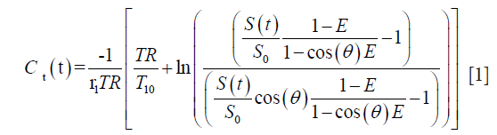
where E=e−TR/T10, r1 is the relaxivity of Gd chelate and θ is the acquisition FA.
AIF methods
The extended Tofts model (described below) requires that Cp, the concentration-time course of contrast agent in the vascular compartment is modelled by an arterial input function (AIF) which reflects the blood supply to the examined tissue. The analysis protocol can be set to use a subject-specific AIF by direct measurement, or a generic mathematic function.
Subject-specific AIF
For a better reproducibility, we implemented a semi-automated search algorithm to generate a locally optimal AIF. The method consists first of a user-defined box that delimits the search region to the input vessels. By using the ImageJ GUI, the task is assisted by an automatic display of the subtraction series presenting the maximal arterial enhancement, this helps the operator to locate easily the vascular structure before defining the box. Then the search algorithm identifies all voxels above a signal intensity threshold (by default 90% of the whole maximum), and using a region growing method, extends the selection in the whole imaging volume entering in the threshold. Next, the Gd concentrations under the selection were corrected to plasma concentrations using:
where by default, the hematocrit Hct is 0.45, but is adjustable in GUI. Then, Cp is calculated using Eq. [1], by assuming an arterial blood T10 of 1,440 ms.
A mathematical modelling of this measured AIF is then calculated using bi-exponential (by default), Orton (18) or mixed model (19):

with D (mmol/kg) the dose of contrast agent, t0 the arrival time in tissue, a1, a2 describing the exponential components amplitude with decay m1, m2, and c simulating the bolus dispersion effect, which equals 0 for bi-exponential, 1 for Orton and any other values for mixed models.
The purpose of this modelling is to produce an AIF free of pulsatile and body motion artifact. All options are let open, including the possibility to choose a standard AIF (below), or the model-free measurement, depending on the study design. This should be set by special consensus in the study protocol.
Standard and population-averaged AIF
If AIF cannot be sampled adequately, a more robust parameter estimate can be achieved by using a population-averaged AIF. From the literature, we optionally included for different range of temporal resolution (TS) 3 commonly used bi-exponential AIF {c=0 in Eq. [2]} obtained from healthy general population:
- Weinmann (20): (TS >20 s) a1 =3.99 kg/L, a2 =4.78 kg/L, m1 =0.144 min−1, m2 =0.0111 min−1.
- Fritz-Hansen (21): (6< TS <20 s) a1 =24 kg/L, a2 =6.2 kg/L, m1 =3.0 min−1, m2 =0.016 min−1.
- Parker (22): (TS <6 s) a1 =65 kg/L, a2 =13 kg/L, m1 =4.9 min−1, m2 =0.08 min−1.
A custom designed AIF can also be set in the analysis protocol.
Fitting algorithm and strategy
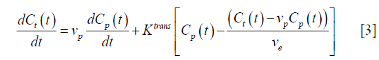
The general consensus for clinical trials is to apply the general bi-compartmental PK model described by Tofts et al. (23). In theory, the model considers the exchange between plasmatic and EES compartments within the capillary endothelium acting as a symmetric semi-permeable membrane. Therefore, under the assumption that the contrast agent is well-mixed in the blood plasma, the equilibrium is described by:
For a bi-exponential AIF model (2), the analytic solution of this differential equation is:

where kep =Ktrans/Ѵe is symmetric exchange rate of contrast agent across the capillary wall.
This time equation directly relates the measured concentration data to model parameters Ktrans, Kep and Ѵp, as well as t0, which have to be extracted using a non-linear fitting algorithm (bellow).
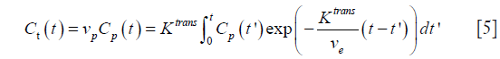
For any forms of AIF model, the general solution of (3) is written:
and usually, it is calculated using deconvolution techniques via the transfer function:
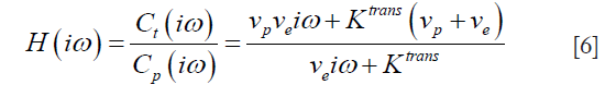
where iω is the variable in frequency domain.
In time or in frequency domain, two fitting routines that can be set freely in the analysis protocol have been implemented in C++ for rapid pixel-wise estimation of the model parameters. We included the commonly used Levenberg-Marquardt (LM) algorithm (24) and adapted the BOBYQA algorithm (25) which was initially written in FORTRAN. What makes the difference is the way in which the iterative steps minimize the χ2 to approach the global best-fit: the LM is a “line search” method which determines directionally the value of fitting parameters, whereas BOBYQA uses the trust region algorithm to minimize χ2 within small regions surrounding the current estimate of the solution and is less likely to find local minima, but is more computationally demanding.
Report of error estimate
Estimates of uncertainty are reported using RMS (root mean square) error map for each fitting parameter. Additionally, all relevant steps in the fitting process (number of iterations, χ2, uncertainty on parameter estimate, fit failures…) can be inspected in a text file for QA or debugging purpose.
Parametric color maps
The pre-contrast images are used for fusion with overlay colors. The analysis protocol contains flexible color cut-offs for each output parameters described above. These cut-offs should be pre-defined as the standard deviation SD in normal like tissue involved in the tumour type, i.e., by measuring them in breast normal glandular tissue, or arbitrarily in the peripheral normal zone of the prostate, so that sub-normal voxels can be detected and classified into 4 color-coded subsets: blue-green-red for parameter values exceeding 1SD-2SD-3SD, and below 1SD no color is attributed. As a result of this definition, subset0 is the whole histogram volume, subsets1 include all the color-coded voxels, subset2 cumulate the green and red, subset3 is red. These cut-offs act as “scaling” or “clustering” purpose, and do nothing to change the quantification results, but have consequent impact on the computer-assisting method described next.
Viewing and reporting
The GUI (Figure 1) is composed of multiple images stacks which allows easy 4-dimensional inspection of parametric mapping in synchronization with the subtraction images, and auxiliary windows for tools, in-line curve display of enhancement curve over 3×3 voxels cursor, and segmentation results. Segmentations can be performed semi-automatically on the tumour total volume and on hot spot ROI, and can be inspected and readjusted manually in consistence with an edit base validation protocol.

The “hot-spot” method differs from the classical assessment in that the parameter calculations are not averaged over a user-dependent ROI, but rather the user locates a color-coded seed-point from which a region growing algorithm segments a contiguous region that most highly characterizes the tumour. With this method, the hot-spot result is the average of parameter values in the segmented voxels, and is likely to be more reproducible.
In the total volume method, the whole tumour is enclosed inside a user-defined bounding box using assistance of orthogonal views. Parameter values in the resulted selection are then plotted using single- or bi-parameters (Ktransvs. Kep) histograms, showing the classification of voxels in subsets. Functional volume response can also be assessed on the blended histograms, and is proposed as an approach to describe quantitatively the functional changes in tumour along follow-up.
Quality performance validation
The initiative to provide synthetic DCE-MRI data is already being undertaken by Buckley (15) and the QIBA group. For our validation, both phantoms were used, the difference is that the Buckley data simulates a realistic breast tumour, but requires to be converted to DICOM images, whereas the QIBA data is a ready-for-use DICOM data set, except that parameter space in low values of Ktrans may be less typical of tumour characteristics. The rationale behind this extreme condition could be to provide a test that allows the estimate of uncertainty and quantitation limit, and to handle the occurrence of fitting failure, as Ktrans =0 min−1 or extremely low is ill-conditioned, so precluding any precision for Ѵe or Kep in the PK model.
The QIBA data consists of 2 sets of DICOM part 10 synthetic noise-free images corresponding to the basic Tofts and the extended Tofts model. To test basic Tofts, we used the QIBA v06 RevC phantom provided by RSNA (26). The simulation parameters are: 0.5 s resolution time, 1,321 sampling, 30° FA, 5 ms TR, 1,000 ms T10 in tissue, 1,440 ms T10 in blood, 45% hematocrit. Injection of contrast agent occurred at 60 seconds, assuming a T1 relaxivity of the gadolinium contrast agent of 4.5 mmol−1 sec-1. The test image is organized as a top and a bottom 50×10 pixels trips between which patches of 10×10 pixels are allocated for combinations of Ktrans and Ѵe in the following scheme: Ktrans varies along Y-axis over (0.01, 0.02, 0.05, 0.1, 0.2, 0.35) min−1 and Ѵe takes values (0.01, 0.05, 0.1, 0.2, 0.5) along X-axis. The top-left 10×10 pixels strip also contains the peak of the vascular region and the time label and the top-right 25×10 pixels correspond to ill-conditioning (Ktrans =0, Ѵe =0.5). Finally, the vascular region is the bottom 50×10 pixels strip of the image.
For the extended Tofts phantom, we used the dcemri_testdata_v2 provided by RSNA (27). Related to the first phantom, differences in the parameterization are: 0.5 s resolution time, 661 sampling and 25° FA. The data contains 10×10 pixels to patch each combination of Ktrans, Ѵe and Ѵp in the following scheme: Ktrans varies along X-axis over (0, 0.01, 0.02, 0.05, 0.1, 0.2) min−1, Ѵe takes values (0.1, 0.2, 0.5) recurrently along Y-axis, while Ѵp takes (0.001, 0.005, 0.01, 0.02, 0.05, 0.1) for each recurrence of Ѵe. The vascular region is the bottom 60×20 pixels strip of the image.
Buckley’s data has two sets, one simulating the breast tumour and the other the brain meningioma response, both consisting in an AIF and 13 concentration curves using different combinations of Ktrans, Ѵe and Ѵp, with a resolution time of 1 s and 301 samplings. In this work, we present the results for breast data with an extension of the original parameter space by 2 additional curves with different Ѵe, giving 1 AIF and 15 combinations for the extended Tofts model (Figure 2). To obtain the DCE-MRI images compatible with current clinical use, we generated a dynamic set of phantom images as well as a set of variable FA images for T1 mapping. The concentration data were first converted to MR signal intensities as described by the Bloch equation of spoiled gradient-echo sequence. Each time-intensity curve was patched into 64×64 pixels, giving a 2562 phantom image and, repeating this allocation for each time points, we obtained the dynamic series images. Subsequently, variable experimental conditions that could affect the performance of the PK quantification software can be incorporated. The final phantom can include customizable perturbation extends towards the image noise, the tissue native T1, the overall onset time, the time delay between arterial input and tissue vasculature, and the measurement protocol (time resolution, repetition time, echo time, FA). In the first experiment, we incorporated 4 tissue T10 (300, 600, 900 and 1,200 ms) arranged 2×2 per patch, and assumed an equilibrium magnetization of 5,000, 30° FA, 4.63 ms TR, 1,440 ms T10 in blood and 45% hematocrit. In the second experiment, a noise of σ =0.2 was added.

In our routine workflow, TumourMetrics has now been evaluated as a diagnostic aid tool for multi-parametric assessment of tumours in prostate, breast and head and neck. We also made the software available to the European MR section of EORTC Imaging Group, and at the time of writing, a multi-centric trial (EORTC 90111) is under our central analysis. The last demonstration is a case which shows the concept for clinical application.
For all experiments, we used the subject-specific AIF with deconvolution method (as suggested in the QIBA profile) and the Bobyqa fitting algorithm which showed the best results in the tested parameter space of phantoms. In the fitting process, the values of the parameters were constrained within upper and lower bounds of (0.001, 1.8) for Ktrans, (0.01, 1.0) for Ѵe, and if applicable (0.001, 1) for Ѵp. RMS errors and intraclass correlation coefficients (ICCs) were calculated to determine the bias and the absolute agreement between estimates and true parameters value. A 3.4 GHz Intel Core i7-2600 running on Windows 7 was used.
Results
QIBA basic Tofts data
The computation time to fit all the voxels was about 8 s. Figure 3 presents a scaled color map of the estimates and the associated errors expressed in % difference to known truth values. The % errors on Ktrans varied within (−15.2, 5.7), with a RMS error of 1.9%. Largest errors occurred for 2 points in the region of low Ѵe values. % errors for Ѵe were within (−15.3, 5.4) with RMS error of 2.2%, and were largest for 3 points in the region of high Ktrans. In this tested parameter space, both parameters were correlated to true values with ICCs >0.995.

QIBA extended Tofts data
The computation time was 52 s. As shown in Figure 4, the % error to known truth was from (−8, 23) for Ktrans, (−27, 50) for Ѵe and (−4.6, >100) for Ѵp. In the same order, the RMS error was 0.9%, 23% and 0.7% with ICCs of 0.997, 0.76 and 0.998. Largest fit errors could be explained by ill-fitting condition at low Ktrans values, except that this strong dependence between Ktrans and Ѵe had little influence on Ѵp, for which the error was rather overemphasized when expressed relatively to very low reference values. Also, the equilibrium magnetization used to simulate these data was relatively low, thus resulting in bad discretization of low signal, and increased the uncertainty of Ѵe estimate as pointed by the poor R coefficient. Ktrans and Ѵp didn’t suffer from this effect because their estimation relies predominantly on the initial high intensities part of enhancement curves.

Buckley breast data
A complete data set including 2 optimized FAs images was generated. The value of these FAs was determined according to DESPOT1 by assuming a T1 of 900 ms in tissue and an acquisition TR of 5.5 ms. The computation time to fit the 2562 voxels was about 164 s. Color map images representing the measured parameter values and the associated % error in noise-free and noise-added cases are shown in Figure 5, while the quantification results can be compared in Figure 6.


In the noise-free case measured on tissue T1 of 900 ms, the % error to known truth was from (−15, 7.9) for Ktrans, (−45, 4.6) for Ѵe and (−49, 29,200) for Ѵp. In the same order, the RMS error was 2.1%, 3.2% and 8.2% with ICCs of 0.94, 0.89 and 0.87. In the Ktrans parameter space, excepted for slight overestimation in 2 extreme conditions (Ktrans very low and Ѵp highest), all estimates were systematically underestimated with a maximum error in the region of low Ѵp values. In the Ѵe parameter space, the estimates matched well their true value except when Ktrans is very low, situation already met previously. Next for Ѵp, again the largest overestimated error was related to its very low simulated value, so there is no substantive concern, but the underestimation related to low Ktrans values should be much more significant, when related to the results for Ktrans, because this shows that even with a resolution time of 1 s, the extended Tofts model wasn’t accurate enough in resolving the ambiguous perfusion and permeability meaning of Ktrans. So, we think that when using the extended Tofts model, the interpretation of Ktrans should be carefully related to Ѵp in terms of dependence.
Next for the determination of T1, the values matched the true data very accurately within a range of 0.3 to 1.44 s, scoring a maximum error of −2.8%, RMS of 0.87 and ICC of 0.999. At 1.6 s, the linearity began to be impaired with an error of −12%. The effect of the tissue native T1 on the accuracy of PK parameters is presented by the error bars in Figure 6A, which shows that the influence exists, but caused minor errors compared to PK model fitting errors.
Finally, a noise of σ =0.2 was added to the phantom to test the precision of our quantification. The parametric maps were analyzed using the ROI selection tools supplied by our GUI. The parameter values in the ROI were averaged in the corresponding patch and reported with the associated standard deviation (SD) in Figure 6B. The results showed no significant difference between the noise-free values and the noise-added means, and the variances expressed as SD ×100/true value indicated that a noise SD of 5 (1/σ) propagated a typical error of the order of 10% on the PK parameter estimates. Also, the influence of noise on T1 determination was to a lesser extend similar, scoring a variance of 6% (Figure 5C).
Example with clinical data
We report here a case from EORTC 90111-24111 multicenter trial relating metabolic response after 2 weeks of treatment with neo-adjuvant afatinib in squamous cell carcinoma of the head and neck. Morphologic conventional MRI, diffusion weighted imaging (DWI) and DCE-MRI were acquired at baseline and after treatment 1 day before surgery with respect to a standardized imaging guideline. The analysis protocol was setup to include individual AIF measurement, T1 mapping, noise filter, the extended Tofts model and the BOBYQA fitting algorithm. The DCE-MRI data was acquired with a resolution time of 3.9 s, sampling 64 series with an imaging matrix of 1922 pixels ×20 slices. The computation time to process all the 737,280 voxels was about 260 s. The resulted parametric response maps were assessed using the parameter values measured in hot-spot ROI and total volume histogram clustered by a cutoff value of 0.3 for Ktrans and 0.5 for Kep as described above. Figure 7 shows the analysis reports at baseline and after treatment from the same operator. Despite the semi-automated segmentation method intended to reduce the observer variability in the selection of the input vessels, the AIF differed significantly between the two visits. Such individual variations in AIF measurement has been reported (28,29), and should be independent of operator, especially since the 2 segmentations appeared very similar. In this example, the analysis with hot- spot showed minor increase of Ktrans (2%), whereas Ѵe decreased by 18%. When accessed by the parametric volume change, the tumour size decreased globally, except in the high Ktrans and higher Kep values. At the same time, the conventional morphologic evaluation showed a discreet reduction of the tumour size (1.7 cm × 2 cm vs. 1.5 cm × 1.6 cm). These findings suggest heterogeneous changes in the tumour vascularity, but in the context of this trial, we are not able to conclude what represents the therapeutic meaning of these changes. This is our first experience using the TumourMetrics software in multicenter clinical trial, with the purpose first to validate the reliability and the usability of this analysis tool in clinical practice and multicentric clinical research and, if the condition is satisfied, to validate the potential use of DCE-MRI as a biomarker of treatment response.

Discussion
Globally, our quantification method estimated the parameters accurately, unless there are extreme circumstances where Ktrans meets a small Ѵe <0.05, and vice-versa when Ѵe gathers with very small Ktrans <0.01. The situation between Ktrans and Ѵp is that they are competing against each other when the balance is becoming unequal, while keeping their respective proportionality towards true values. So, we recommend special caution when using the extended Tofts in the clinical achievable time resolution (3 s for a best), because the conflict between Ktrans and Ѵp is increasing with the time resolution (30,31), and both parameters should be reported. For this reason, the QIBA profile recommends the use of basic Tofts. We cannot say in the scope of this study if using the basic model to quantify high resolution time data if Ѵp exists is more accurate or clinically relevant, given that the tumours vascularization is an essential micro-environmental indication for anti-vascular and radiotherapy treatments. Large clinical trials are needed to validate the approach, and this is what the present project would be aimed. In the meantime, simulation studies with our numeric phantom are under investigation to help understanding this issue.
Most clinical CAD software applies a smoothing filter on DCE-MRI data to reduce the noise effect, thus our software also incorporated this option in the setting of analysis protocol. As shown in Figure 6C, the filter globally reduced the % variance to values lesser than the errors on parameters.
Regarding the advantages of TumourMetrics, we acknowledge that in clinical practice, other analysis tools such as those provided by MR scanner vendors may be fully or partly compliant with QIBA and could be equally efficient as for quality performance. At our knowledge, there was not QIBA test data validation using these clinical solutions that has been published to make the comparison. In a recent study, Beuzit et al. compared the accuracy and reproducibility among five of mostly used clinical software using in-house simulated data and clinical data (32). Their results showed significant errors in calculated parameters and poor inter-software reproducibility. This variability may be mainly explained by the different methods used to process all steps of parameters quantification, given that some of these were not fully compliant with the QIBA recommendations.
In our work, we used publicly available simulated data. Assuming that the method used by Beuzit et al. for the generation of in-house simulated data was the same, a rough comparison of ICCs could be made: for our Buckley data ICCs was 0.94 for Ktrans and 0.89 for Ѵe, while the overall ICCs yielded by Beuzit et al. were respectively 0.5 and 0.67.
Conclusions
We still emphasize that our objective was not to demonstrate that our software is doing better than other commercial or non-commercial software, but to provide a reliable freely accessible DCE-MRI post-processing software that firstly ensures the compliance with the standardization of analysis methods, and secondly achieves an easy integration of DCE-MRI in routine clinical practice, but also as a clinical research tool. In our knowledge, there is no open source and freely accessible software application that can achieve these objectives by dealing with the needs of community radiologists.
The package includes both the PK quantification of DCE-MRI data and a straightforward interpretation GUI which limits the inter-operator variability. The software has been first designed for easy integration into the clinical workflow. At our radiology department, TumourMetrics runs as a plugin in the diagnostic workstation and provides means for complete interpretation of breast and prostate studies without the need of dedicated workstation. By selecting the patient study from the PACS viewer, a single click starts the application with the computation of parametric maps. The process time generally falls under one minute, so that reading physician will stay focused on the same investigation, and without transition, the results obtained are interpreted using our home-developed GUI for visualization, ROI and VOI analysis and reporting. For the quality assessment, the DICOM structure info of parametric maps records all parameters of methods used for PK quantification like AIF, FAs for T1 mapping or fitting algorithm. For a full clinical integration, all results and analysis reports are signed using user login, and automatically transferred to the PACS.
To address the issue of standardization in both DCE-MRI quantification and analysis in ROI and VOI, our software can be set to be fully compliant with the widely accepted QIBA DCE-MRI Profile, since set up to facilitate the standardization, development, and validation of quantitative imaging biomarkers.
Finally, the reliability of our results has been demonstrated using publicly available simulated data, providing an important basis for multicenter reproducibility of the method. Moreover, a quantification protocol can be made fit for purpose to ensure prospectively a strict consistency between each center participating in a clinical trial: this has a major interest in oncology and also in series focusing on rare diseases.
We think that this open source solution gives the possibility to develop easily additional approaches to tumour measurements, i.e., improving the ROI or volume segmentation tools or new quantification methods to evaluate the heterogeneity of tumours, as well as heterogeneous response to treatment.
Acknowledgements
None.
Footnote
Conflicts of Interest: The authors have no conflicts of interest to declare.
Ethical Statement: All procedures performed in studies involving human participants were in accordance with the ethical standards of the institutional and/or national research committee and with the 1964 Helsinki declaration and its later amendments or comparable ethical standards. This article does not contain any studies with animals performed by any of the authors. For this type of study formal consent was not required.
References
- Veltman J, Stoutjesdijk M, Mann R, Huisman HJ, Barentsz JO, Blickman JG, Boetes C. Contrast-enhanced magnetic resonance imaging of the breast: the value of pharmacokinetic parameters derived from fast dynamic imaging during initial enhancement in classifying lesions. Eur Radiol 2008;18:1123-33. [Crossref] [PubMed]
- Brix G, Kiessling F, Lucht R, Darai S, Wasser K, Delorme S, Griebel J. Microcirculation and microvasculature in breast tumors: pharmacokinetic analysis of dynamic MR image series. Magn Reson Med 2004;52:420-9. [Crossref] [PubMed]
- Shukla-Dave A, Lee NY, Jansen JF, Thaler HT, Stambuk HE, Fury MG, Patel SG, Moreira AL, Sherman E, Karimi S, Wang Y, Kraus D, Shah JP, Pfister DG, Koutcher JA. Dynamic contrast-enhanced magnetic resonance imaging as a predictor of outcome in head-and-neck squamous cell carcinoma patients with nodal metastases. Int J Radiat Oncol Biol Phys 2012;82:1837-44. [Crossref] [PubMed]
- O'Connor JP, Jackson A, Parker GJ, Jayson GC. DCE-MRI biomarkers in the clinical evaluation of antiangiogenic and vascular disrupting agents. Br J Cancer 2007;96:189-95. [Crossref] [PubMed]
- QIBA DCE-MRI Technical Committee: DCE-MRI Profile v.1.0, Jul. 1 2012. Available online: http://www.rsna.org/uploadedFiles/RSNA/Content/Science_and_Education/QIBA/DCE-MRI_Quantification_Profile_v1%200-ReviewedDraft%208-8-12.pdf
- Leach MO, Brindle KM, Evelhoch JL, Griffiths JR, Horsman MR, Jackson A, Jayson GC, Judson IR, Knopp MV, Maxwell RJ, McIntyre D, Padhani AR, Price P, Rathbone R, Rustin GJ, Tofts PS, Tozer GM, Vennart W, Waterton JC, Williams SR, Workman P. Pharmacodynamic/Pharmacokinetic Technologies Advisory Committee, Drug Development Office, Cancer Research UK. The assessment of antiangiogenic and antivascular therapies in early-stage clinical trials using magnetic resonance imaging: issues and recommendations. Br J Cancer 2005;92:1599-610. [Crossref] [PubMed]
- Recommendations from 2004 NCI workshop (pdf). Available online: http://imaging.cancer.gov/images/Documents/14a39040-dad1-46f8-bf88bae2e7401ebe/DCE_RecommendationfromNov2004NCIWorkshop(2).pdf
- Daniel P. Barboriak Laboratory, Duke University School of Medicine. Toppcat, T1-weighted Perfusion Imaging Parameter Calculation Toolkit. Available online: http://dblab.duhs.duke.edu/modules/dblabs_topcat/
- Schmid WB. Quantitative analysis of dynamic contrast-enhanced and diffusion-weighted magnetic resonance imaging for oncology in R. J Stat Software 2011;44:1-29.
- Ferl GZ. DATforDCEMRI: an R package for deconvolution analysis and visualization of DCE-MRI data. J Stat Software 2011;44:1-18. [Crossref]
- Smith DS, Li X, Arlinghaus LR, Yankeelov TE, Welch EB. DCEMRI.jl: a fast, validated, open source toolkit for dynamic contrast enhanced MRI analysis. PeerJ 2015;3:e909. [Crossref] [PubMed]
- Dale BM, Jesberger JA, Lewin JS, Hillenbrand CM, Duerk JL. Determining and optimizing the precision of quantitative measurements of perfusion from dynamic contrast enhanced MRI. J Magn Reson Imaging 2003;18:575-84. [Crossref] [PubMed]
- Kershaw LE, Buckley DL. Precision in measurements of perfusion and microvascular permeability with T1-weighted dynamic contrast-enhanced MRI. Magn Reson Med 2006;56:986-92. [Crossref] [PubMed]
- Schabel MC, Parker DL. Uncertainty and bias in contrast concentration measurements using spoiled gradient echo pulse sequences. Phys Med Biol 2008;53:2345-73. [Crossref] [PubMed]
- Buckley DL. Uncertainty in the analysis of tracer kinetics using dynamic contrast-enhanced T1-weighted MRI. Magn Reson Med 2002;47:601-6. [Crossref] [PubMed]
- Klein S, Staring M, Murphy K, Viergever MA, Pluim JP. elastix: a toolbox for intensity-based medical image registration. IEEE Trans Med Imaging 2010;29:196-205. [Crossref] [PubMed]
- Deoni SC, Peters TM, Rutt BK. Determination of optimal angles for variable nutation proton magnetic spin-lattice, T1, and spin-spin, T2, relaxation times measurement. Magn Reson Med 2004;51:194-9. [Crossref] [PubMed]
- Orton MR, d'Arcy JA, Walker-Samuel S, Hawkes DJ, Atkinson D, Collins DJ, Leach MO. Computationally efficient vascular input function models for quantitative kinetic modelling using DCE-MRI. Phys Med Biol 2008;53:1225-39. [Crossref] [PubMed]
- Balvay D, Ponvianne Y, Claudon M, Cuenod CA. Arterial input function: Relevance of eleven analytical models in DCE-MRI studies. IEEE International Symposium on Biomed Imaging 2008:600-3.
- Weinmann HJ, Laniado M, Mützel W. Pharmacokinetics of GdDTPA/dimeglumine after intravenous injection into healthy volunteers. Physiol Chem Phys Med NMR 1984;16:167-72. [PubMed]
- Fritz-Hansen T, Rostrup E, Larsson HB, Søndergaard L, Ring P, Henriksen O. Measurement of the arterial concentration of Gd-DTPA using MRI: a step toward quantitative perfusion imaging. Magn Reson Med 1996;36:225-31. [Crossref] [PubMed]
- Parker GJ, Roberts C, Macdonald A, Buonaccorsi GA, Cheung S, Buckley DL, Jackson A, Watson Y, Davies K, Jayson GC. Experimentally-derived functional form for a population-averaged high-temporal-resolution arterial input function for dynamic contrast-enhanced MRI. Magn Reson Med 2006;56:993-1000. [Crossref] [PubMed]
- Tofts PS, Brix G, Buckley DL, Evelhoch JL, Henderson E, Knopp MV, Larsson HB, Lee TY, Mayr NA, Parker GJ, Port RE, Taylor J, Weisskoff RM. Estimating kinetic parameters from dynamic contrast-enhanced T(1)-weighted MRI of a diffusible tracer: standardized quantities and symbols. J Magn Reson Imaging 1999;10:223-32. [Crossref] [PubMed]
- Press WH, Teukolsky SA, Vetterling WT, Flannery BP. Numerical Recipes in C. Second Edition. Cambridge University Press, 1992:683-7.
- Powell MJ. The BOBYQA algorithm for bound constrained optimization without derivatives. Department of Applied Mathematics and Theoretical Physics, Cambridge University. DAMTP 2009/NA06. Retrieved 2014-02-14.
- Quantitative Imaging Data Warehouse (QIDW). Available online: https://www.rsna.org/QIDW/
- QIBA_v4 Extended Tofts, 2009.04.16, D. P. Barboriak Lab, Duke University. Available online: https://sites.duke.edu/dblab/qibacontent/
- Mendichovszky IA, Cutajar M, Gordon I. Reproducibility of the aortic input function (AIF) derived from dynamic contrast-enhanced magnetic resonance imaging (DCE-MRI) of the kidneys in a volunteer study. Eur J Radiol 2009;71:576-81. [Crossref] [PubMed]
- Ashton E, Raunig D, Ng C, Kelcz F, McShane T, Evelhoch J. Scan-rescan variability in perfusion assessment of tumors in MRI using both model and data-derived arterial input functions. J Magn Reson Imaging 2008;28:791-6. [Crossref] [PubMed]
- Henderson E, Rutt BK, Lee TY. Temporal sampling requirements for the tracer kinetics modeling of breast disease. Magn Reson Imaging 1998;16:1057-73. [Crossref] [PubMed]
- Heisen M, Fan X, Buurman J, van Riel NA, Karczmar GS, ter Haar Romeny BM. The influence of temporal resolution in determining pharmacokinetic parameters from DCE-MRI data. Magn Reson Med 2010;63:811-6. [Crossref] [PubMed]
- Beuzit L, Eliat PA, Brun V, Ferré JC, Gandon Y, Bannier E, Saint-Jalmes H. Dynamic contrast-enhanced MRI: Study of inter-software accuracy and reproducibility using simulated and clinical data. J Magn Reson Imaging 2016;43:1288-300. [Crossref] [PubMed]

